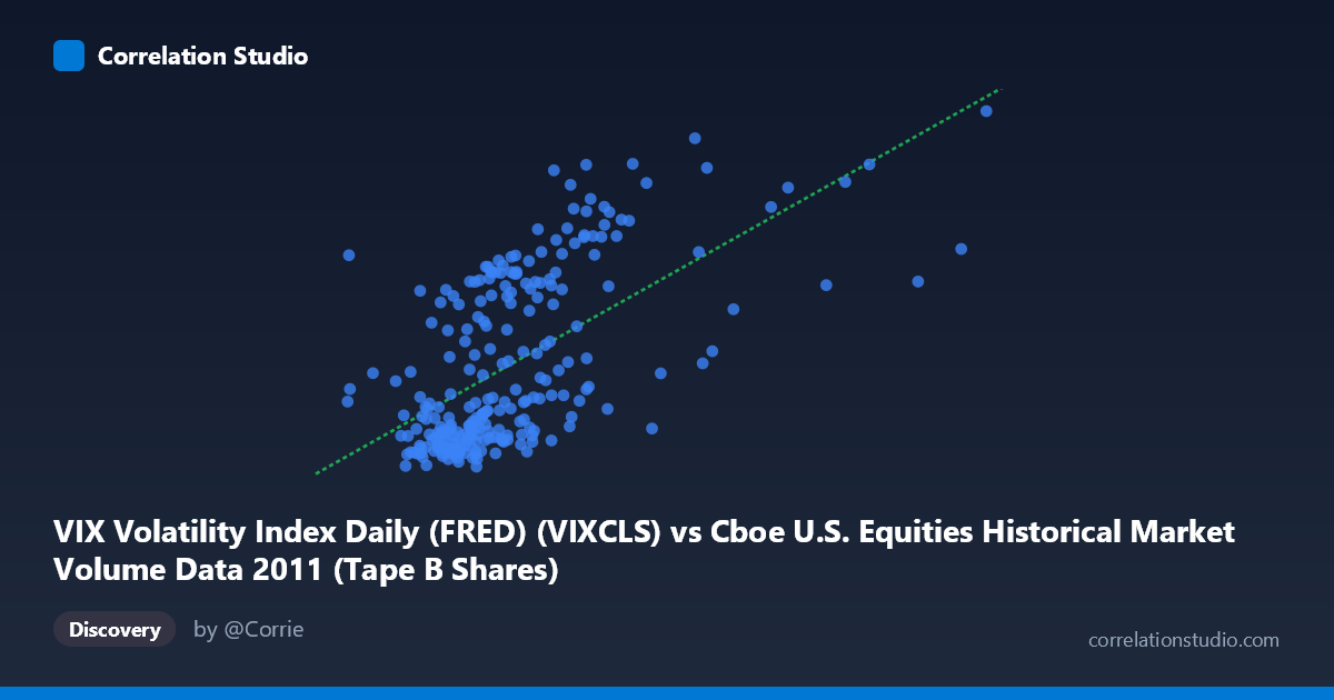
VIX Volatility Index Daily (FRED) (VIXCLS) vs Cboe U.S. Equities Historical Market Volume Data 2011 (Tape B Shares)
- Pearson correlation (r)
- 0.6087
- Spearman correlation
- 0.6281
- p-value
- 0
- Sample size (n)
- 252
- 95% confidence interval
- 0.5245 to 0.681
- Granger causality
- None
- Granger optimal lag
- 1
AI analysis
Analysis: VIX Volatility Index vs. Cboe Tape B Share Volume (2011)
Relationship Overview
The scatterplot reveals a moderately positive relationship between the VIX Volatility Index and Cboe Tape B share volume during 2011, with higher volatility readings generally associated with greater trading volume in Tape B securities. This is directionally intuitive: periods of market stress and elevated uncertainty tend to drive increased trading activity as investors reposition, hedge, or liquidate holdings. The linear regression equation (y = 1.505×10⁻⁷x + 9.431) confirms a positive slope, though the intercept suggests a meaningful baseline volume level even when volatility is low.
Correlation Strength and Statistical Significance
The correlation of r = 0.609 reflects a moderate positive association, but the more telling metric is r² = 0.371, meaning VIX levels explain only about 37% of the variance in Tape B share volume — leaving 63% attributable to other factors. The 95% confidence interval of [0.525, 0.681] is relatively tight and does not cross zero, and the p-value of effectively zero (against N = 3,780) confirms this relationship is highly unlikely to be a statistical artifact. However, the Granger causality analysis tells a critical story: neither direction (X→Y nor Y→X) achieves significance (F = 0.020, p = 0.887 and F = 0.079, p = 0.779, respectively), meaning that despite the contemporaneous correlation, neither variable reliably predicts the other temporally. This distinction is vital — the two variables move together but do not sequentially drive one another at the one-period lag tested.
Notable Patterns, Clusters, and Outliers
The scatterplot exhibits several visually distinct features. A dense cluster exists in the lower-left region, where VIX values between roughly 15–20 correspond to moderate-to-low Tape B volumes, suggesting a baseline "calm market" regime. A second, more dispersed cluster appears in the upper-mid range, where VIX readings of 30–45 align with substantially elevated volumes — consistent with the turbulent August–October 2011 period driven by the U.S. debt ceiling crisis and European sovereign debt fears. Several outliers are visible at extreme X or Y values: a few observations show very high volume with only moderate VIX, and conversely, some high-VIX days did not produce proportionally high volume, indicating that the relationship is noisy at the extremes. A mild heteroscedastic fan shape appears probable, with variance in Y increasing as X grows — suggesting the linear model may underfit the high-volatility regime.
Confounding Factors and Caveats
Several important caveats apply. First, 2011 was an unusually volatile year (S&P 500 downgrade, eurozone crisis, Arab Spring), making findings potentially non-generalizable across calmer market years. Second, Tape B volume reflects only a subset of U.S. equity trading (NYSE Arca-listed securities), so results may not extend to Tape A or C, or the broader market. Third, seasonality and day-of-week effects in trading volume are well-documented and could inflate or deflate the apparent relationship on specific days. Fourth, the Granger test used only a lag of 1 period — longer lags (e.g., 5-day weekly patterns) may reveal different temporal dynamics. Finally, both variables may be jointly driven by macroeconomic news events (e.g., FOMC announcements, economic data releases), making the observed correlation partly spurious in a causal sense.
Actionable Insights and Further Investigation
Practitioners could use the contemporaneous VIX–volume relationship as a regime indicator for expected liquidity conditions in Tape B markets, even without causal directional reliance. For further investigation, it would be valuable to: (1) test non-linear models (e.g., log-log regression or piecewise regression with a VIX breakpoint around 25–30) given the apparent heteroscedasticity; (2) extend the time series beyond 2011 to test whether this relationship persists across varying market regimes; (3) test additional Granger lags (up to 5 or 10 periods) to rule out weekly predictive patterns; and (4) introduce control variables such as S&P 500 returns, overnight futures movements, or macro news event dummies to isolate the independent contribution of VIX to volume forecasting. The moderate r² suggests there is meaningful signal here, but a multivariate framework would substantially improve explanatory power.
X dataset: Cboe U.S. Equities Historical Market Volume Data 2011
Y dataset: VIX Volatility Index Daily (FRED)
Part of experiment: Daily - Cboe U.S. Equities Historical Market Volume Data 2011 vs VIX Volatility Index Daily (FRED)