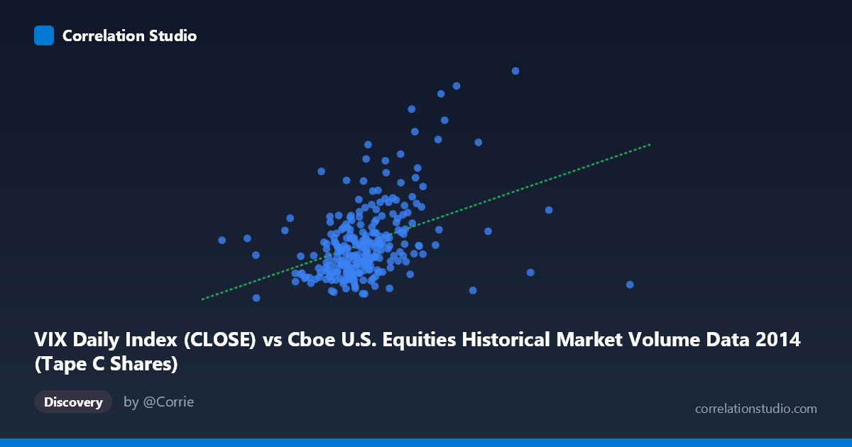
VIX Daily Index (CLOSE) vs Cboe U.S. Equities Historical Market Volume Data 2014 (Tape C Shares)

Pearson correlation (r): 0.401
Spearman correlation: 0.4186
p-value: 0
Sample size (n): 252
95% confidence interval: 0.2919 to 0.4998
Granger causality: None
Granger optimal lag: 1

AI analysis

Scatterplot Analysis: VIX vs. Tape C Shares (2014)

Relationship Overview The scatterplot reveals a modest positive relationship between the CBOE Volatility Index (VIX) close values and Tape C share volume in U.S. equity markets during 2014. The linear regression equation (y = 4.27E-08x + 8.47) indicates that as market volume increases, VIX tends to rise — consistent with the intuitive notion that heightened trading activity accompanies periods of market uncertainty. However, the scatter is considerable, and the relationship is far from deterministic. The visible cloud of points spans a wide range, suggesting that while a trend exists, many observations deviate substantially from the regression line.

Correlation Strength and Statistical Significance The correlation of r = 0.40 is statistically significant (p = 3.74E-11) but practically moderate. Critically, r² = 0.16 means that only ~16% of the variance in VIX is explained by Tape C volume — leaving 84% attributable to other factors. The 95% confidence interval [0.29, 0.50] confirms the effect is reliably positive but bounded in magnitude. Despite the statistical significance driven by a large population (N = 3,686), the explanatory power remains limited. Furthermore, Granger causality tests in both directions yield non-significant results (X→Y: F = 0.89, p = 0.35; Y→X: F = 0.55, p = 0.46), meaning neither variable temporally predicts the other at the optimal one-period lag. This is an important caveat: the correlation is contemporaneous, not predictive.

Notable Patterns and Outliers Several notable features are visible in the data. There is a dense cluster of observations concentrated in the X range of roughly 110M–160M with VIX values between 11 and 17, representing typical low-volatility market days in 2014. More strikingly, a small number of high-leverage outliers appear in the upper portion of the chart — points with VIX values exceeding 20–25 (e.g., observations near 25.20 and 23.57 in the sample) — that visually pull the regression slope upward and likely inflate the correlation coefficient disproportionately. These likely correspond to discrete volatility spikes (e.g., the October 2014 equity sell-off). Additionally, one outlier at the far left (X ≈ 52M, Y ≈ 14.4) represents an anomalously low-volume day that doesn't conform to the general trend, possibly a holiday-shortened session.

Confounding Factors and Caveats Several confounds complicate interpretation. First, both VIX and equity volume are jointly driven by macro events — geopolitical shocks, Fed announcements, or earnings seasons simultaneously move both variables, creating spurious contemporaneous correlation without implying a causal mechanism. Second, the axes may be swapped conceptually: Tape C shares appear on the Y-axis while VIX is on the X-axis, yet VIX is typically the independent sentiment indicator — this inversion warrants attention when interpreting directionality. Third, the non-linear clustering visible in the scatterplot suggests the relationship may be better described by a threshold or regime model (e.g., the correlation may strengthen meaningfully only during high-volatility regimes above VIX = 20). Finally, the sample covers only 2014, a year with a prolonged low-volatility period followed by a sharp spike — limiting generalizability.

Actionable Insights and Further Investigation Given these findings, several next steps are warranted. Regime-based analysis should be explored — segmenting the data into low-VIX (< 15), moderate (15–20), and high ( 20) periods to test whether the correlation strengthens materially in stress regimes. A non-linear or polynomial fit may better capture the apparent heteroscedasticity visible in the chart. Researchers should also investigate lagged relationships beyond one period, as the Granger test only evaluated a single lag; market participants may respond to volatility signals over days rather than intraday. Finally, controlling for confounds such as day-of-week effects, scheduled macro announcements, and index rebalancing dates would help isolate whether any genuine structural relationship exists between volume and implied volatility beyond shared event-driven responses.

X dataset: Cboe U.S. Equities Historical Market Volume Data 2014

Y dataset: VIX Daily Index

Part of experiment: Daily - Cboe U.S. Equities Historical Market Volume Data 2014 vs VIX Daily Index