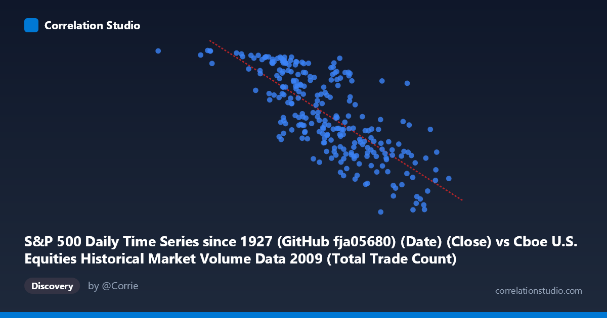
S&P 500 Daily Time Series since 1927 (GitHub fja05680) (Date) (Close) vs Cboe U.S. Equities Historical Market Volume Data 2009 (Total Trade Count)

Pearson correlation (r): -0.7592
Spearman correlation: -0.7697
p-value: 0
Sample size (n): 252
95% confidence interval: -0.8071 to -0.7014
Granger causality: X → Y
Granger optimal lag: 10

AI analysis

Analysis: S&P 500 Close Price vs. U.S. Equities Total Trade Count (2009)

Relationship Overview The scatterplot reveals a moderately strong negative relationship between the S&P 500 closing price (X-axis) and the total trade count across U.S. equities exchanges (Y-axis) throughout 2009. As the S&P 500 index level increases, the number of discrete trades executed daily tends to decrease. This is a counterintuitive but meaningful pattern: when markets were depressed (early 2009 lows near 629–700 range), trading activity in terms of raw trade counts was at its highest, while recovery toward year-end corresponded with fewer, presumably larger or more consolidated, transactions.

Correlation Strength and Statistical Significance The Pearson correlation of r = -0.7592 indicates a substantial negative association, and the R² of 0.5764 means that approximately 57.6% of the variance in daily trade counts is statistically explained by the S&P 500 price level. The remaining ~42% reflects other influences not captured by this linear model. The 95% confidence interval of [-0.8071, -0.7014] is relatively narrow and sits entirely in negative territory, providing strong statistical confidence that the true population correlation is meaningfully negative. The p-value of effectively zero confirms this is not a chance finding across the n=252 trading days sampled from a population of N=3,232 records. Critically, the Granger causality analysis identifies a unidirectional predictive relationship: X (S&P 500 price) Granger-causes Y (trade count) at an optimal lag of 10 trading periods (F=2.015, p=0.033), while the reverse direction fails to reach significance (F=1.620, p=0.102). This suggests that S&P 500 price movements have modest but statistically meaningful forward-looking predictive power over trade counts approximately two calendar weeks later, though the F-statistic is modest and should not be overstated as a strong causal mechanism.

Notable Patterns, Clusters, and Outliers Several structural features are visible in the data. There is a clear high-density cluster around the mid-range X values (2,000,000–3,200,000 in the encoded date/price space) with trade counts concentrated between 850–1,100, suggesting the bulk of 2009 trading days fell in a recoverable mid-market regime. The lower-left region contains notable outliers with very low X values (e.g., 629,671 corresponding to crisis-era lows) yet extremely high trade counts (~1,126), consistent with the panic-driven fragmentation of orders typical of bear-market bottoms. Conversely, the upper-right extreme (X ~4,134,002, Y ~770) represents late-2009 recovery levels with markedly suppressed trade counts. The regression line (y = -0.000146508x + 1338.79) fits this trend reasonably, but there is visible heteroscedasticity: scatter around the regression line is wider at lower X values, suggesting that during volatile, low-price periods, trade count behavior becomes less predictable from price alone.

Confounding Factors and Interpretive Caveats Several important caveats temper interpretation. First, 2009 was a historically anomalous year, spanning the tail of the Global Financial Crisis trough (March 2009 S&P lows near 666) and a dramatic recovery rally, meaning this correlation may reflect a regime-specific artifact rather than a generalizable structural relationship. Second, the rise in trade counts at lower price levels likely reflects algorithmic and high-frequency trading (HFT) fragmentation — during volatile, fearful markets, institutional players break large orders into many small ones, inflating trade counts independently of price. Third, market structure changes within 2009 itself (regulatory shifts, exchange fee changes, dark pool activity) could introduce non-stationarity. Fourth, while Granger causality is present, it is a test of predictive precedence, not true causality — both variables may be jointly driven by a latent factor such as VIX (implied volatility) or investor sentiment indices.

Actionable Insights and Further Investigation Practitioners and researchers should consider several follow-up directions. Incorporating VIX as a control variable would help isolate whether the price–trade count relationship survives after accounting for volatility regime, potentially revealing whether the negative correlation is a direct price effect or a volatility-mediated one. Given the 10-period Granger lag, a short-term trading signal framework could be tested: sustained price increases might predict reduced market microstructure noise (fewer trades) roughly two weeks forward, with implications for execution strategy and liquidity forecasting. It would also be valuable to replicate this analysis across multiple years (2007–2010) to determine whether this pattern is crisis-specific or persistent. Finally, decomposing trade count by exchange venue (Cboe, NYSE, NASDAQ, TRFs) would clarify whether the effect is concentrated in specific market centers, potentially revealing structural rather than behavioral explanations for the observed negative correlation.

X dataset: Cboe U.S. Equities Historical Market Volume Data 2009

Y dataset: S&P 500 Daily Time Series since 1927 (GitHub fja05680) (Date)

Part of experiment: Daily - Cboe U.S. Equities Historical Market Volume Data 2009 vs S&P 500 Daily Time Series since 1927 (GitHub fja05680) (Date)