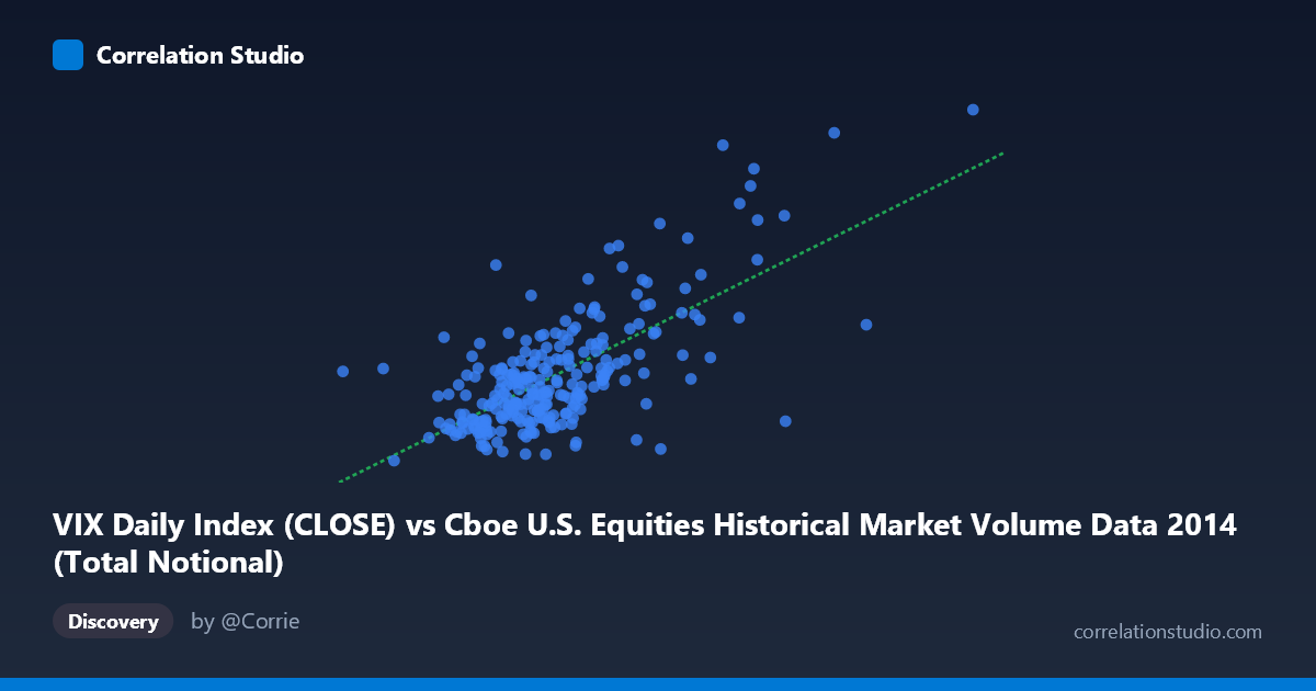
VIX Daily Index (CLOSE) vs Cboe U.S. Equities Historical Market Volume Data 2014 (Total Notional)

Pearson correlation (r): 0.6915
Spearman correlation: 0.5705
p-value: 0
Sample size (n): 252
95% confidence interval: 0.621 to 0.7509
Granger causality: None
Granger optimal lag: 1

AI analysis

Scatterplot Analysis: VIX vs. Total Market Notional Volume (2014)

Relationship Overview

The scatterplot reveals a moderately positive relationship between the CBOE Volatility Index (VIX) daily close values and total U.S. equities notional trading volume throughout 2014. As VIX rises, market notional volume tends to increase in tandem — a relationship that aligns intuitively with market microstructure theory: elevated fear or uncertainty (captured by VIX) typically drives heavier trading activity as participants react to perceived risk, rebalance portfolios, and execute hedges. The linear regression equation (y = 4.71×10⁻¹⁰x + 5.796) confirms a positive slope, meaning each unit increase in notional volume is associated with a measurable uptick in the VIX level.

Correlation Strength and Statistical Significance

The correlation is moderate-to-strong at r = 0.692, with r² = 0.478, meaning approximately 47.8% of the variance in VIX is explained by notional trading volume — a meaningful but incomplete picture. The remaining 52% is attributable to other factors entirely outside this bivariate frame. The 95% confidence interval for r [0.621, 0.751] is relatively tight and excludes zero, and the p-value is effectively zero, confirming this correlation is highly unlikely to be a statistical artifact given the sample of 252 paired observations. However, the Granger causality results are notably absent: neither X→Y (F=1.13, p=0.288) nor Y→X (F=0.22, p=0.640) achieves significance at lag 1. This means that while the two variables move together contemporaneously, neither reliably predicts the other's future values — ruling out a straightforward lagged predictive relationship and suggesting the correlation is driven by shared simultaneous drivers rather than one variable leading the other.

Notable Patterns, Clusters, and Outliers

The scatterplot exhibits a few visually distinct features worth noting. The bulk of observations cluster in a moderately tight band between VIX values of roughly 11–17 and notional volumes in the 13–22 billion range, reflecting the relatively calm, low-volatility environment that characterized much of 2014. However, there are clear high-leverage outliers in the upper-right quadrant — points with VIX readings approaching 23–26 and notional volumes near 27–37 billion. These likely correspond to specific stress episodes in late 2014 (e.g., the October 2014 market selloff triggered by Ebola fears and global growth concerns), when VIX spiked sharply and trading volumes surged simultaneously. One notable outlier at approximately (7.69B, 14.37) sits far left of the main cluster at a low volume with a mid-range VIX, potentially representing a trading anomaly or data irregularity. These extreme points likely exert disproportionate influence on the correlation coefficient, inflating r beyond what the core cluster alone would produce.

Confounding Factors and Interpretive Caveats

Several important caveats apply to this analysis. First, reverse causality is plausible: VIX is itself derived from options market pricing, which is intimately linked to trading volumes; the correlation may be partially tautological. Second, common drivers — such as macroeconomic announcements, Federal Reserve policy signals, geopolitical events, or earnings seasons — could simultaneously elevate both VIX and notional volume without one causing the other. Third, the dataset covers only calendar year 2014, a relatively tranquil market period with one notable volatility episode, limiting generalizability to other regimes (e.g., 2008 or 2020). Fourth, notional volume reflects both price levels and share counts, so rising notional values could partly reflect price appreciation during high-VIX periods rather than purely increased trading intensity. The axis labels also appear to be swapped in the statistical notes (VIX is on Y, notional on X), which warrants verification before drawing directional conclusions.

Actionable Insights and Further Investigation

Practitioners and researchers should consider several follow-up avenues. Regime-based segmentation — splitting the data into calm versus stressed periods using a VIX threshold (e.g., <15 vs. ≥20) — could reveal whether the relationship holds uniformly or is driven primarily by tail episodes. Testing longer Granger causality lags (beyond 1 period) may uncover delayed predictive dynamics missed at lag 1. Incorporating intraday data or volume broken down by trade type (retail vs. institutional, block trades) could disentangle the mechanisms at play. A multivariate model controlling for S&P 500 returns, Fed announcement days, and earnings calendar effects would clarify how much of the shared variance is truly attributable to the VIX-volume relationship versus common shocks. Finally, replicating this analysis across multiple years including crisis periods would test whether the r ≈ 0.69 finding is stable or regime-dependent — critical information for any trading strategy or risk model that relies on this relationship.

X dataset: Cboe U.S. Equities Historical Market Volume Data 2014

Y dataset: VIX Daily Index

Part of experiment: Daily - Cboe U.S. Equities Historical Market Volume Data 2014 vs VIX Daily Index