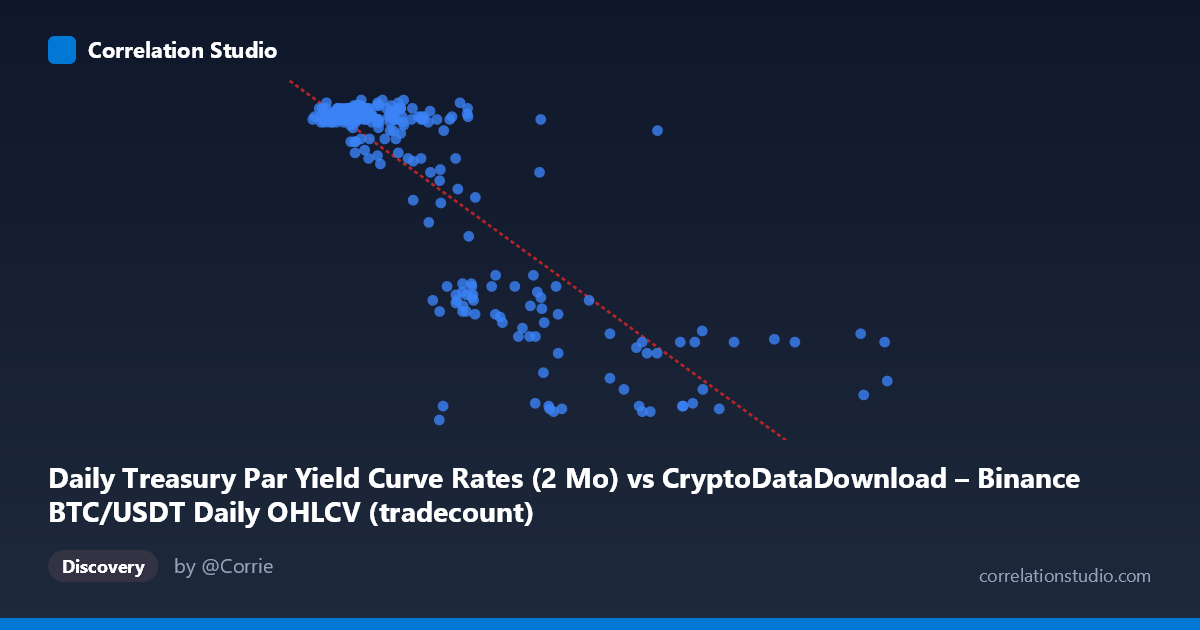
Daily Treasury Par Yield Curve Rates (2 Mo) vs CryptoDataDownload – Binance BTC/USDT Daily OHLCV (tradecount)
- Pearson correlation (r)
- -0.8231
- Spearman correlation
- -0.6694
- p-value
- 0
- Sample size (n)
- 250
- 95% confidence interval
- -0.8594 to -0.7786
- Granger causality
- X → Y
- Granger optimal lag
- 1
- Time coverage
- 2024-01-02 to 2024-12-31
AI analysis
Analysis of Variable Relationship
Note on labeling: The axis labels appear swapped from their descriptions — the X-axis values (900K–12M range) and Y-axis values (4.39–5.54 range) don't match "Treasury 2-Mo Yield" and "tradecount" naming conventions. Based on the actual data ranges, X appears to be a trade/volume-type metric and Y appears to be the yield series (values clustering 4.4–5.5, consistent with 2024 short-term Treasury yields). The analysis below treats the data as given numerically.
1. Overall Relationship
The scatterplot reveals a strong negative, non-linear relationship between X and Y. As X increases from ~1M to ~12M, Y declines from roughly 5.5 down to ~4.4. The relationship is not a simple straight line — it shows a steep drop-off pattern: Y stays clustered tightly near 5.45–5.55 for X values below ~4M, then declines sharply and more variably as X exceeds ~4M, consistent with a curved (possibly logarithmic or inverse) decay rather than pure linearity.
2. Strength, Direction, and Statistical Confidence
The correlation coefficient (r = -0.823) indicates a strong inverse relationship, with r² = 0.6775 meaning roughly 68% of the variance in Y is statistically explained by X — a substantial but not complete explanatory power (32% remains unaccounted for). The 95% CI [-0.859, -0.779] is tight and entirely negative, and the p-value ≈ 0 confirms this relationship is highly unlikely to be due to chance at n=250. Practically, this is a robust, reproducible association.
The Granger causality results add a temporal dimension: X Granger-causes Y (F=7.63, p=0.0062) at lag 1, while the reverse (Y→X) is not significant (p=0.373). This suggests X's past values have predictive power for future Y values, but not vice versa — implying a unidirectional, time-lagged dynamic rather than pure contemporaneous correlation. This is meaningful for forecasting but does not establish causation in the mechanistic sense.
3. Patterns and Outliers
Two distinct regimes are visible: a dense, low-variance cluster at low X (roughly X < 4M, Y ≈ 5.4–5.55) representing the majority of points, and a sparser, more scattered tail at high X (X 8M) where Y drops to 4.4–4.7. The transition zone (X ≈ 4M–8M) shows the most scatter and mixed values (Y from 4.7 to 5.1), suggesting a regime change or threshold effect rather than smooth continuous decay. No extreme outliers break the pattern, but the high-X tail is thin (few points support the extrapolation beyond X ≈ 9M).
4. Confounders and Caveats
Given the mismatched axis descriptions, a key caveat is data provenance uncertainty — verify that X/Y are correctly mapped to their intended series before drawing domain conclusions. Both series likely share a common time trend across 2024 (macro conditions, seasonality), which can inflate correlation without direct causal linkage — classic spurious correlation via a shared time trend risk. Additionally, the non-linear shape means the linear r²=0.68 may understated the true explanatory relationship (or reflect two separate sub-populations/regimes being pooled).
5. Suggested Next Steps
1. Confirm variable identity/units — resolve the axis-label mismatch before publishing conclusions. 2. Test non-linear models (log, power, or piecewise regression) given the visible curvature — likely to improve fit over the linear r²=0.68. 3. Detrend both series (e.g., first-difference or control for date) to rule out spurious correlation from shared temporal trends before trusting Granger causality results. 4. Investigate the regime-shift zone (X ≈ 4–8M) — segment the data and check if a structural break or threshold model fits better than continuous correlation. 5. Use the Granger result cautiously as a leading indicator in forecasting models, but validate out-of-sample given single-lag testing and moderate F-statistic (7.63).
X dataset: CryptoDataDownload – Binance BTC/USDT Daily OHLCV
Y dataset: Daily Treasury Par Yield Curve Rates
Part of experiment: Bitcoin - CryptoDataDownload – Binance BTC/USDT Daily OHLCV vs Daily Treasury Par Yield Curve Rates