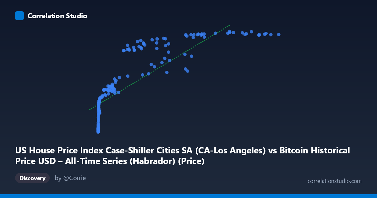
US House Price Index Case-Shiller Cities SA (CA-Los Angeles) vs Bitcoin Historical Price USD – All-Time Series (Habrador) (Price)
- Pearson correlation (r)
- 0.8346
- Spearman correlation
- 0.9705
- p-value
- 0
- Sample size (n)
- 189
- 95% confidence interval
- 0.7855 to 0.8733
- Granger causality
- None
- Granger optimal lag
- 9
- Time coverage
- 2010-08-01 to 2026-04-01
- Recomputed on refreshed data
- 2026-10-22 (r was 0.8303)
AI analysis
Analysis: Bitcoin Price vs. US House Price Index (Case-Shiller, LA)
1. What the visualization reveals
The scatterplot shows a strongly non-linear, monotonically increasing relationship between Bitcoin's historical price (X) and the Case-Shiller Los Angeles home price index (Y). At low Bitcoin prices (under ~$1,000), the HPI values cluster tightly in the 160-260 range with a steep initial rise. As Bitcoin price increases into the thousands and tens of thousands, the HPI values climb into the 300-450 range but with visibly diminishing marginal increases — the curve flattens noticeably above ~$60,000. This concave, logarithmic-looking shape (rapid early growth, then saturation) rather than a straight line is the dominant visual feature.
2. Strength, direction, and statistical caveats
The Pearson correlation (r = 0.83) indicates a strong positive linear association, with r² = 0.689 meaning the linear model explains about 69% of the variance in Y — leaving nearly a third unexplained. The 95% CI [0.78, 0.87] is fairly tight and the p-value is effectively 0, so the correlation itself is statistically robust and not a fluke of sampling. However, statistical significance here should not be read as evidence of a causal or even directly meaningful economic relationship — it largely reflects that both series have trended upward over the same historical period (2010–2026). Critically, the Granger causality tests show no significant predictive direction in either direction (X→Y: p=0.79; Y→X: p=0.77) even at an optimal lag of 9 periods. This strongly suggests the correlation is not driven by one variable temporally leading or forecasting the other — it's more consistent with two independent trending series that happen to co-move over time (a classic spurious-correlation pattern with time series).
3. Notable patterns and features
The data show three rough regimes: (a) a "micro-cap" cluster where X < 100 and Y sits near 160-175 (Bitcoin's earliest, near-worthless days), (b) a middle zone (X ~ 100–10,000) where HPI rises steadily from ~180 to ~280, and (c) a high-X regime (X 20,000) where HPI plateaus around 400-450 despite huge further increases in Bitcoin price (e.g., X jumping from 60,000 to 118,670 while Y barely moves from 431 to 441). This ceiling effect in Y is the strongest evidence against a linear fit and explains why Spearman's ρ exceeds Pearson's r — a log or power-law transform of X would likely fit much better than the raw linear model (y = 0.0026x + 241).
4. Confounding factors and caveats
The most obvious confound is shared time trend: Bitcoin's price and US housing prices have both risen substantially from 2010-2026, driven by largely unrelated macro forces (crypto adoption/speculation vs. housing supply, interest rates, demographics, monetary policy). Both series are also non-stationary (trending), which mechanically inflates correlation coefficients between unrelated trending series — a well-known issue in time-series statistics. Additionally, Bitcoin's extreme scale range (0.06 to 118,670) means the correlation is heavily influenced by a few high-leverage points at the upper end; log-transforming X would likely change both the fit and the apparent strength of association.
5. Suggested next steps
Before drawing any economic conclusion, analysts should: (a) refit using log(X) or a saturating/logistic function given the visual and Spearman-vs-Pearson evidence of non-linearity; (b) test both series for stationarity (e.g., ADF test) and consider differencing or working with returns/growth rates rather than levels, then re-run correlation and Granger tests on the stationary series; (c) explicitly model the shared time trend (e.g., detrend both series or include a time variable) to see if the relationship survives; and (d) given the null Granger causality result, avoid framing this as a predictive or causal relationship — it's best presented as a co-trending pattern, useful perhaps for narrative/illustrative purposes but not for forecasting one series from the other.
X dataset: Bitcoin Historical Price USD – All-Time Series (Habrador)
Y dataset: US House Price Index Case-Shiller Cities SA
Part of experiment: Bitcoin - Bitcoin Historical Price USD – All-Time Series (Habrador) vs US House Price Index Case-Shiller Cities SA