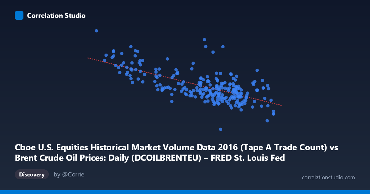
Cboe U.S. Equities Historical Market Volume Data 2016 (Tape A Trade Count) vs Brent Crude Oil Prices: Daily (DCOILBRENTEU) – FRED St. Louis Fed (DCOILBRENTEU)
- Pearson correlation (r)
- -0.6729
- Spearman correlation
- -0.6012
- p-value
- 0
- Sample size (n)
- 251
- 95% confidence interval
- -0.7354 to -0.599
- Granger causality
- None
- Granger optimal lag
- 10
- Time coverage
- 2016-01-04 to 2016-12-30
- Recomputed on refreshed data
- 2026-10-22 (r was -0.6729)
AI analysis
Analysis: Cboe U.S. Equities Trade Count vs. Brent Crude Oil Prices (2016)
Relationship Overview
The scatterplot reveals a moderate-to-strong negative relationship between Cboe U.S. equities trade count (X) and Brent crude oil prices (Y) across 251 trading days in 2016. As equity trade volume increases, Brent crude prices tend to decline — and conversely, lower trade activity coincides with higher oil prices. The linear regression equation (y = -29,755.5x + 2,690,680) quantifies this inverse slope: each unit increase in trade count is associated with a decrease of roughly 29,756 units in crude price. Visually, the data points form a discernible downward-sloping cloud, most dense in the mid-range of both variables, with a notable spread suggesting meaningful but imperfect predictability.
Correlation Strength and Statistical Framing
The Pearson correlation of r = -0.6729 indicates a moderately strong negative association. More critically, r² = 0.4528 means that approximately 45.3% of the variance in Brent crude prices is statistically explained by equity trade count — a substantial share, though it equally means ~55% of variance lies elsewhere. The 95% confidence interval of [-0.7354, -0.5990] is relatively tight and does not cross zero, and the p-value of effectively 0 (from N = 3,622) confirms this correlation is highly unlikely to be a chance artifact. However, the Granger causality tests yield no significant directional predictive relationship in either direction (X→Y: F = 0.755, p = 0.672; Y→X: F = 0.760, p = 0.668) at the optimal 10-period lag. This is a crucial distinction: while the contemporaneous correlation is strong, neither variable reliably predicts the other temporally, which substantially limits any causal interpretation or forecasting application.
Notable Patterns, Clusters, and Outliers
Several structural features warrant attention. The data exhibits a dense central cluster roughly between trade counts of 44–50 and crude prices of 1,100,000–1,500,000, suggesting these represent typical 2016 market conditions. There is a visually striking upper-left cluster of outliers — points like (26.01, 2,497,318), (27.59, 2,013,606), (31.83, 1,859,406), and (33.01, 1,860,056) — representing days with very low trade counts and unusually high crude prices. These extreme low-volume, high-price observations disproportionately drive the negative slope and may correspond to early 2016 when oil prices were recovering from multi-year lows amid thinner equity market activity. At the other extreme, points like (53.01, 1,000,524) anchor the lower-right region. There is also a suggestion of heteroscedasticity: variance in Y appears larger at lower X values, which could slightly inflate the apparent correlation strength.
Confounding Factors and Interpretive Caveats
This correlation almost certainly reflects shared temporal dynamics rather than a direct causal mechanism. Both variables are time-series observed across 2016, and crude oil prices underwent a significant recovery during that year (from ~$27/barrel in January to ~$55 by year-end), while equity trading volumes followed their own cyclical and seasonal patterns. Temporal autocorrelation in both series is the most likely confound — early-year low-price, low-volume conditions versus late-year higher-price, higher-volume conditions could manufacture a spurious cross-variable correlation. Additionally, macro events (OPEC decisions, U.S. election, Fed policy) likely drove both variables simultaneously, acting as common external drivers rather than one causing the other. The axis labels also appear swapped in the dataset metadata (the X-axis description references oil prices while the Y-axis references trade count), which should be verified to ensure the regression direction is correctly interpreted.
Actionable Insights and Further Investigation
Given the absence of Granger causality, practitioners should not attempt to use trade count as a leading indicator for crude prices (or vice versa) in any trading or risk model — the relationship is contemporaneous at best. Further investigation should include: (1) decomposing both time series to remove trend and seasonality before re-examining correlation, to test whether the relationship holds beyond shared directional drift; (2) examining whether the relationship is driven predominantly by the January–February 2016 outlier cluster, using subsample or rolling-window correlations; (3) introducing explicit control variables such as VIX (equity volatility), USD index, and OPEC production data to isolate whether any residual relationship survives; and (4) testing non-linear specifications, given the visible curvature hint and heteroscedasticity in the scatter, which may better capture the true functional form between these two market variables.
X dataset: Brent Crude Oil Prices: Daily (DCOILBRENTEU) – FRED St. Louis Fed
Y dataset: Cboe U.S. Equities Historical Market Volume Data 2016
Part of experiment: Daily - Brent Crude Oil Prices: Daily (DCOILBRENTEU) – FRED St. Louis Fed vs Cboe U.S. Equities Historical Market Volume Data 2016