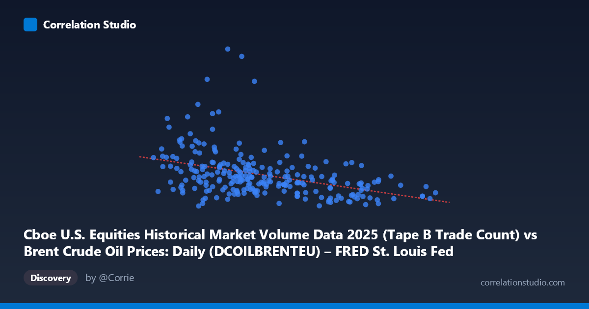
Cboe U.S. Equities Historical Market Volume Data 2025 (Tape B Trade Count) vs Brent Crude Oil Prices: Daily (DCOILBRENTEU) – FRED St. Louis Fed (DCOILBRENTEU)
- Pearson correlation (r)
- -0.4017
- Spearman correlation
- -0.4566
- p-value
- 0
- Sample size (n)
- 246
- 95% confidence interval
- -0.5016 to -0.2912
- Granger causality
- None
- Granger optimal lag
- 10
AI analysis
Scatterplot Analysis: Cboe Tape B Trade Count vs. Brent Crude Oil Price
1. Overall Relationship
The scatterplot reveals a modest negative relationship between Cboe U.S. Equities Tape B trade counts (X-axis, ranging roughly 60–83 units) and Brent Crude Oil prices (Y-axis, ranging from ~$407K to ~$1.72M in the scaled units shown). The fitted regression line (y = -14,758.9x + 1,686,290) slopes downward, suggesting that on days when equity trade counts are higher, Brent crude prices tend to be lower, and vice versa. However, the scatter around this line is substantial, indicating the linear model captures only a fraction of the actual data variability.
2. Correlation Strength, Direction, and Statistical Framing
The Pearson correlation of r = -0.40 confirms a statistically significant but practically moderate negative association. Critically, R² = 0.161, meaning that only about 16% of the variance in crude oil prices is explained by trade count levels — leaving roughly 84% attributable to other factors entirely. The 95% confidence interval for r spans [-0.50, -0.29], which is meaningfully narrow given n = 246, confirming the negative direction is reliable but also confirming the effect is not large. The p-value of 5.9 × 10⁻¹¹ is highly significant, reflecting the large underlying population (N = 4,805) rather than necessarily implying strong practical effect size. Most importantly, Granger causality testing finds no significant predictive directionality in either direction (X→Y: F = 0.59, p = 0.82; Y→X: F = 0.87, p = 0.56), meaning neither variable meaningfully predicts the other across time, even at the optimal 10-period lag. The correlation, while real, does not reflect a temporal forecasting relationship.
3. Notable Patterns, Outliers, and Non-Linear Features
Several notable features stand out in the data: - High-leverage outliers are visible in the upper-left region, most strikingly the point near (66.13, 1,718,887) — the single highest Y-value in the sample — and (62.78, 1,152,125) and (64.86, 1,178,999), all clustering at low trade counts with anomalously high crude prices. These outliers likely exert disproportionate influence on the negative slope. - Compression at moderate trade counts (68–73): The bulk of observations cluster in this central band with Y-values concentrated between ~$500K–$750K, suggesting a relatively stable regime for most trading days. - Right-tail sparsity: Points beyond X = 77 (e.g., 83.48 at ~$517K) are rare and tend to have lower crude prices, consistent with the negative trend but too few to be conclusive. - The spread of Y-values appears to fan out at lower X values, hinting at possible heteroscedasticity — lower trade count days show far greater variability in crude prices than higher trade count days.
4. Confounding Factors and Interpretation Caveats
Several important caveats apply:
- Axis label mismatch: The dataset description suggests a possible column-swapping artifact — Tape B trade count appears on the X-axis sourced from the Brent Crude dataset, and vice versa. This warrants careful data verification before drawing any conclusions. - Spurious correlation risk: Equity market volume and crude oil prices are both driven by macro conditions (geopolitical events, OPEC decisions, risk-on/risk-off sentiment, economic data releases). Any observed correlation may reflect shared responses to third-party drivers rather than a direct link. - Temporal confounding: Over a single calendar year (2025), both series may exhibit trending or seasonal behavior that artificially inflates or deflates the measured correlation. - Outlier sensitivity: The three extreme high-Y observations (particularly the ~$1.72M point) likely pull the regression slope substantially; removing them could materially weaken or alter the estimated relationship. - Scale ambiguity: The Y-axis values in the hundreds of thousands are unusual for Brent crude prices (typically ~$70–$90/barrel), suggesting these may be notional or aggregated values rather than per-barrel spot prices, complicating direct interpretation.
5. Actionable Insights and Further Investigation
Given the weak explanatory power, absent Granger causality, and potential data labeling concerns, the following steps are recommended:
1. Verify data alignment: Confirm that the column assignments are correct and that the units on both axes are meaningful and consistently scaled — the Y-axis magnitude is inconsistent with typical Brent spot prices. 2. Outlier investigation: Isolate and investigate the three high-Y outliers to determine whether they represent data errors, extreme market events (e.g., geopolitical shocks), or genuine regime breaks. 3. Control for macroeconomic drivers: Introduce control variables (VIX, USD index, OPEC announcements, inventory reports) to test whether the apparent negative correlation survives multivariate adjustment. 4. Non-linear modeling: Given the visual heteroscedasticity and outlier clustering, explore quantile regression or regime-switching models that may better characterize tail behavior. 5. Extend the time series: With only one year of data and no Granger causality detected, a longer panel (5–10 years) would provide much stronger power to detect or rule out any genuine predictive relationship between equity market activity and crude benchmarks.
X dataset: Brent Crude Oil Prices: Daily (DCOILBRENTEU) – FRED St. Louis Fed
Y dataset: Cboe U.S. Equities Historical Market Volume Data 2025
Part of experiment: Daily - Brent Crude Oil Prices: Daily (DCOILBRENTEU) – FRED St. Louis Fed vs Cboe U.S. Equities Historical Market Volume Data 2025