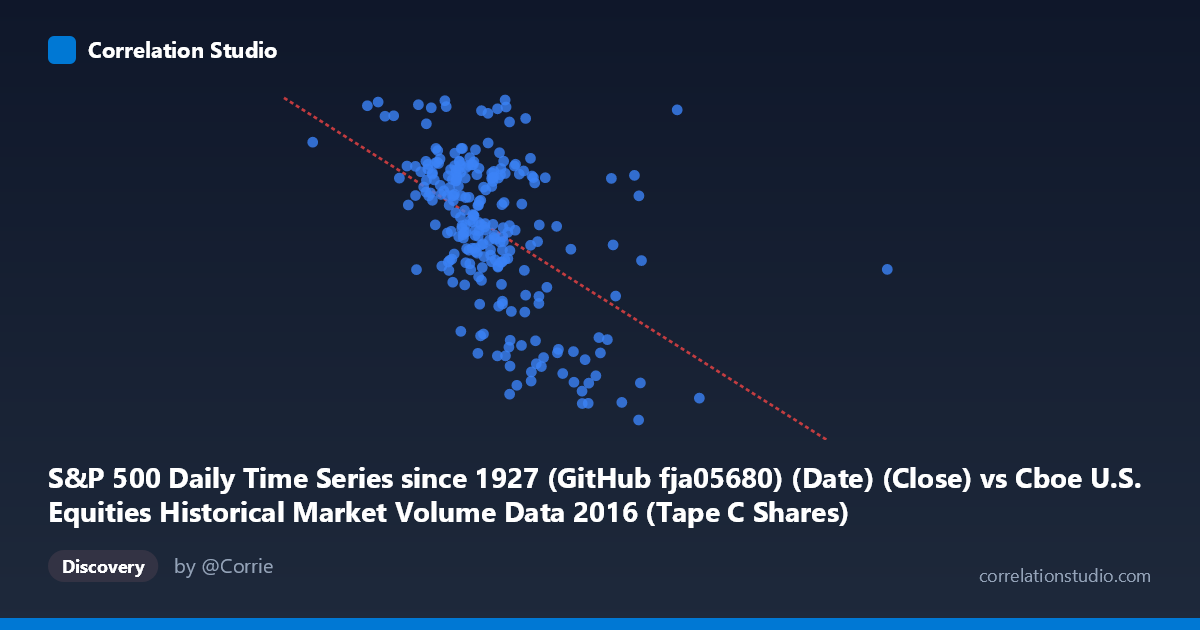
S&P 500 Daily Time Series since 1927 (GitHub fja05680) (Date) (Close) vs Cboe U.S. Equities Historical Market Volume Data 2016 (Tape C Shares)

Pearson correlation (r): -0.5091
Spearman correlation: -0.5
p-value: 0
Sample size (n): 252
95% confidence interval: -0.5952 to -0.4114
Granger causality: None
Granger optimal lag: 4

AI analysis

Analysis: S&P 500 Close Price vs. Cboe Tape C Share Volume (2016)

Relationship Overview The scatterplot reveals a moderate negative relationship between S&P 500 daily closing prices (X-axis) and Cboe Tape C share volume (Y-axis) across 252 trading days in 2016. The linear regression equation (y = -1.8959E-06x + 2346.72) confirms that as the S&P 500 closes at higher price levels, Tape C share volume tends to decline. This is a financially intuitive pattern: during periods of market strength and elevated index levels, trading activity in certain segments can actually decrease as investors hold positions rather than actively trade, reducing turnover volume. The relationship is visible in the data cloud, where higher X values (index levels exceeding ~150 million in the scaled units) tend to cluster toward lower Y values (below ~2,000 shares), while lower index levels correspond to higher volume readings.

Correlation Strength and Statistical Significance The correlation coefficient of r = -0.5091 indicates a moderate negative association, but the explained variance is more sobering: R² = 0.2592 means only ~26% of the variance in Tape C volume is accounted for by S&P 500 price levels, leaving roughly 74% of volume variation unexplained by this single factor. The 95% confidence interval of [-0.5952, -0.4114] is meaningfully narrow and does not cross zero, and with a p-value effectively at 0 across a population of N = 3,622, the correlation is statistically robust and unlikely to be a sampling artifact. However, the Granger causality results are a critical counterpoint: neither direction (X→Y nor Y→X) achieves significance at the optimal 4-period lag (F = 0.9458, p = 0.4381 for X→Y; F = 1.4135, p = 0.2301 for Y→X). This means that while a contemporaneous correlation exists, neither variable reliably predicts the other temporally — the relationship is associative, not predictive in a causal time-series sense.

Patterns, Clusters, and Outliers Several notable features emerge from the sample points. There is a visible upper-left cluster of observations where index values fall in the ~94M–125M range and Tape C volume frequently exceeds 2,150–2,265 shares, consistent with the negative trend. Conversely, data points at higher index values (~150M–175M) tend to show volumes below 1,900, forming a lower-right cluster that anchors the regression line. A few notable outliers deserve attention: the point near (99,790,437; 2,265.18) represents unusually high volume at a relatively low index level, while points around (175,021,320; 1,869.0) and (166,150,058; 1,893.4) show very low volume at elevated price levels. The scatter around the regression line is substantial, suggesting heteroscedasticity — variance in volume appears wider at moderate index levels, narrowing at the extremes. No strong non-linear curvature is apparent, though the wide scatter hints that a simple linear model may be underfitting the true relationship.

Confounding Factors and Caveats Several important caveats temper interpretation. First, Tape C specifically represents NYSE Arca-listed securities, so this volume metric reflects a subset of total market activity rather than aggregate trading — its drivers may differ structurally from broad market dynamics. Second, 2016 was an eventful year (Brexit aftermath, U.S. presidential election in November) that introduced episodic volatility spikes which likely drove volume independently of price levels, potentially inflating or distorting the correlation. Third, the axes may reflect different units or scaling conventions given the dataset crossover (S&P 500 price vs. market volume data), and the very large X-axis values suggest the "Close" column may have been mismatched or represents a running aggregate rather than a simple daily close — warranting data provenance verification. Finally, the absence of Granger causality suggests this correlation may be driven by a common third factor such as macroeconomic conditions, VIX levels, or calendar effects (end-of-quarter rebalancing, options expiration cycles) that simultaneously influence both series.

Actionable Insights and Further Investigation Practitioners should not use S&P 500 price levels alone to forecast Tape C volume — the Granger results make clear there is no reliable temporal predictive edge. Instead, several follow-up analyses are warranted. Incorporating implied volatility (VIX) as a covariate would likely improve explanatory power substantially, since volatility is a known volume driver. A multiple regression or VAR model including VIX, time-of-year dummies, and options expiration indicators could identify whether the negative price-volume relationship persists after controlling for these factors. Segmenting the data by market regime (e.g., pre- vs. post-election) would test whether the correlation is stable or driven by a specific sub-period. Additionally, verifying the data join between the two source datasets is essential before drawing any operational conclusions, as the axis labeling suggests a potentially complex cross-dataset merge that could introduce alignment errors.

X dataset: Cboe U.S. Equities Historical Market Volume Data 2016

Y dataset: S&P 500 Daily Time Series since 1927 (GitHub fja05680) (Date)

Part of experiment: Daily - Cboe U.S. Equities Historical Market Volume Data 2016 vs S&P 500 Daily Time Series since 1927 (GitHub fja05680) (Date)