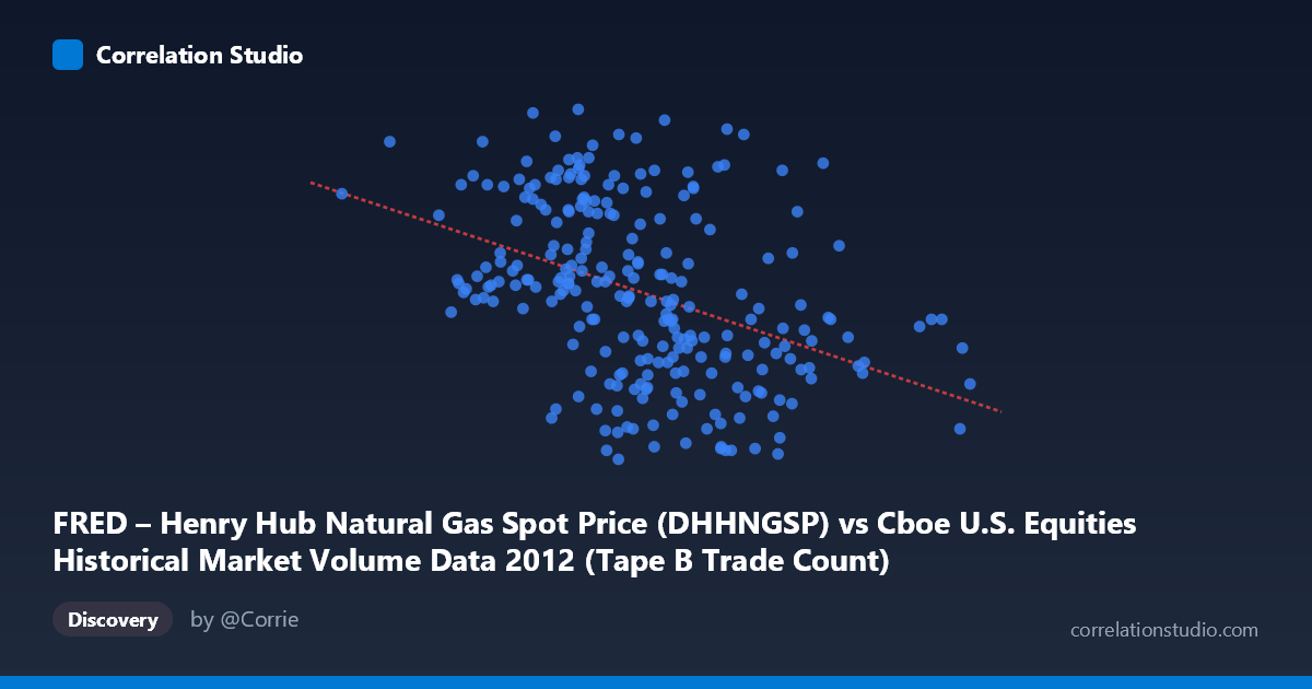
FRED – Henry Hub Natural Gas Spot Price (DHHNGSP) vs Cboe U.S. Equities Historical Market Volume Data 2012 (Tape B Trade Count)
- Pearson correlation (r)
- -0.4093
- Spearman correlation
- -0.4551
- p-value
- 0
- Sample size (n)
- 250
- 95% confidence interval
- -0.5076 to -0.3004
- Granger causality
- None
- Granger optimal lag
- 1
AI analysis
Scatterplot Analysis: Natural Gas Spot Price vs. Cboe Tape B Trade Count (2012)
Relationship Overview
The scatterplot reveals a modest negative relationship between Henry Hub Natural Gas Spot Price (X-axis) and Cboe U.S. Equities Tape B Trade Count (Y-axis) across 250 trading days in 2012. The linear regression equation (y = -4.95×10⁻⁶x + 3.618) describes a downward-sloping trend, indicating that as equity market trade volume (notional value proxy) increases, natural gas spot prices tend to be somewhat lower. Visually, the data points form a diffuse, elongated cloud with considerable scatter around the regression line, reinforcing that the relationship, while statistically detectable, is far from deterministic. The X variable spans a wide range (~$63K to ~$298K), while Y (gas price) clusters predominantly between $2.00 and $3.75/MMBtu, suggesting most trading days fall within a relatively compressed price band.
Correlation Strength and Statistical Framing
The Pearson correlation of r = -0.409 indicates a weak-to-moderate negative association. Critically, r² = 0.167, meaning only 16.7% of the variance in natural gas prices is explained by equity trade count — leaving over 83% attributable to other factors entirely. The 95% confidence interval for r of [-0.508, -0.300] is entirely negative and does not cross zero, and the p-value of 1.63×10⁻¹¹ confirms the correlation is highly statistically significant given n = 250. However, statistical significance here is driven substantially by sample size (N = 3,750 population), and significance should not be conflated with practical or economic importance. Most critically, Granger causality tests find no significant predictive direction in either direction (X→Y: F = 0.757, p = 0.385; Y→X: F = 1.952, p = 0.164), meaning neither variable meaningfully predicts the other's future values at a 1-period lag. This effectively rules out a straightforward temporal causal mechanism.
Notable Patterns, Clusters, and Outliers
Several features stand out within the scatter. A cluster of high gas prices (~$3.40–$3.77/MMBtu) appears predominantly associated with lower-to-mid trade count values (~$100K–$175K range), consistent with the negative slope. Conversely, very low gas prices (~$1.82–$2.00/MMBtu) appear scattered across moderate-to-high trade count values. A handful of notable outliers are visible: one point near (295K, 2.44) represents an extreme equity volume day with an unremarkable gas price, sitting far right of the main cluster and potentially exerting leverage on the regression line. Similarly, points such as (~143K, 3.62) and (~173K, 3.61) represent elevated gas prices that deviate from expected values at those trade counts. The overall spread suggests substantial heteroscedasticity — variance in Y appears somewhat larger at lower X values, which could subtly affect the reliability of the linear fit.
Confounding Factors and Interpretive Caveats
The most significant caveat is that this correlation almost certainly reflects shared seasonal confounding rather than any direct economic linkage. Both equity market volume and natural gas prices have well-documented seasonal patterns in 2012 — gas prices were historically low in early-to-mid 2012 (post-shale boom dynamics) and recovered later in the year, while equity volumes follow their own seasonal rhythms (e.g., lower summer volumes, higher volatility periods). Any co-movement may simply reflect both variables responding independently to calendar effects, macroeconomic conditions (e.g., risk-off periods), or weather patterns rather than influencing each other. Additionally, Tape B specifically represents regional exchange volume (NYSE American, NYSE Arca, etc.), which introduces a narrower equity market signal than total market volume. The absence of Granger causality strongly supports the interpretation that this is a spurious or coincidental correlation mediated by external common drivers.
Actionable Insights and Further Investigation
Given the weak explanatory power and absent Granger causality, practitioners should not use equity trade counts as a predictor of natural gas prices or vice versa in any operational model. However, several avenues merit further investigation: (1) Decompose seasonality from both series and re-test the deseasonalized residuals to determine whether any correlation persists after removing calendar effects; (2) Extend the time horizon beyond 2012 to assess whether this negative relationship is a structural feature or an artifact of a single anomalous year in natural gas markets; (3) Test mediating variables such as VIX (market uncertainty), crude oil prices, or heating/cooling degree days, which may explain both series simultaneously; (4) Explore non-linear models given the visual heteroscedasticity and potential threshold effects at extreme volume levels. The correlation is statistically interesting but economically fragile — further structural analysis is needed before drawing any substantive conclusions.
X dataset: Cboe U.S. Equities Historical Market Volume Data 2012
Y dataset: FRED – Henry Hub Natural Gas Spot Price
Part of experiment: Daily - Cboe U.S. Equities Historical Market Volume Data 2012 vs FRED – Henry Hub Natural Gas Spot Price