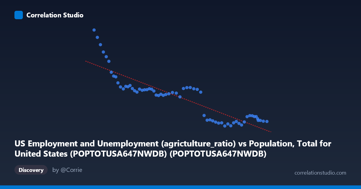
US Employment and Unemployment (agrictulture_ratio) vs Population, Total for United States (POPTOTUSA647NWDB) (POPTOTUSA647NWDB)
- Pearson correlation (r)
- -0.8847
- Spearman correlation
- -0.8695
- p-value
- 0
- Sample size (n)
- 65
- 95% confidence interval
- -0.9283 to -0.8171
- Granger causality
- None
- Granger optimal lag
- 10
- Time coverage
- 1960-01-01 to 2024-01-01
AI analysis
Scatterplot Analysis: US Population vs. Agriculture Employment Ratio
Overview of the Relationship
The scatterplot reveals a strong negative relationship between total US population (X-axis) and the agriculture employment ratio (Y-axis) spanning 1960 to 2024. As the US population has grown from approximately 181 million to 340 million, the share of employment in agriculture has declined dramatically from over 5,400 to around 2,100. The linear regression equation (y = -1.45337E-05x + 6,880.69) captures this inverse trajectory well, describing a consistent long-term structural transformation of the US labor market away from agricultural work as the population expanded and the economy modernized.
Correlation Strength and Statistical Significance
The correlation coefficient of r = -0.8847 indicates a strong negative association, and the R² value of 0.7826 means that roughly 78.3% of the variance in the agriculture employment ratio is statistically explained by total population size. This is a substantial explanatory proportion for a single-variable model applied across six decades of macroeconomic data. The 95% confidence interval for r of [-0.9283, -0.8171] is relatively narrow and sits entirely in negative territory, reinforcing high confidence that the inverse relationship is genuine and not a statistical artifact. The p-value of effectively zero confirms the result is highly statistically significant at any conventional threshold. However, the Granger causality tests tell a critical story: neither X→Y (F = 0.8183, p = 0.6136) nor Y→X (F = 0.8920, p = 0.5502) reaches significance, even at a 10-period optimal lag. This means that while the two variables are strongly correlated, neither one temporally predicts the other in a causal time-series sense — both are almost certainly co-moving products of a common underlying driver rather than causally linked to each other directly.
Patterns, Clusters, and Notable Features
The data points form two visually distinct clusters. The first cluster occupies the lower-left region (population ~180–270 million, agriculture ratio ~3,100–5,500), corresponding roughly to 1960 through the 1990s, where the decline in agriculture ratio was steep but the population base was smaller. The second cluster is concentrated in the upper-right region (population ~280–340 million, agriculture ratio ~2,100–2,500), reflecting the 2000s through 2020s, where the agriculture ratio appears to have plateaued near a floor, compressing the spread of Y values considerably. Several high-leverage outliers are visible at the low-population, high-agriculture-ratio end — notably the point near (180,671,000; 5,458) and (183,691,000; 5,200), likely corresponding to the early 1960s — which exert strong influence on the regression slope. The flattening of Y in the modern cluster hints at a possible non-linear or asymptotic relationship, suggesting the agriculture ratio may be approaching a structural minimum below which it cannot easily fall.
Confounding Factors and Caveats
The most significant caveat is that both variables are primarily driven by time — population grows monotonically with calendar year, and the agriculture employment ratio has declined as a result of mechanization, globalization, and sectoral economic shifts, also trending with time. This creates a classic spurious correlation via shared temporal trend: any two variables with consistent long-term directional trends will appear correlated even if they have no mechanistic connection, which the Granger test results reinforce. The remaining ~21.7% of unexplained variance likely reflects business cycles, policy shifts, commodity price shocks, and measurement changes. Additionally, the Y-axis variable — an agriculture employment ratio — conflates absolute agricultural employment with total labor force size, introducing compositional complexity. Population growth itself may marginally suppress the ratio arithmetically, adding a mechanical component to the correlation that is not economically meaningful.
Actionable Insights and Further Investigation
Researchers should detrend both series (e.g., via first-differencing or removing a common time trend) before drawing any structural conclusions, as the raw correlation almost certainly overstates the direct relationship between population size and agricultural employment share. It would be valuable to model the agriculture ratio against direct economic drivers — mechanization indices, real agricultural wages, trade openness, or rural-urban migration rates — to identify genuine explanatory variables. The apparent plateau in the agriculture ratio below ~2,500 warrants investigation into whether this represents a structural floor tied to food security requirements or subsistence farming. Segmenting the analysis into pre- and post-1990 periods could test whether the relationship has fundamentally changed in character, given the visible clustering behavior. Finally, incorporating state-level or regional disaggregation could reveal heterogeneous dynamics masked by the national aggregate.
X dataset: Population, Total for United States (POPTOTUSA647NWDB)
Y dataset: US Employment and Unemployment
Part of experiment: Yearly - Population, Total for United States (POPTOTUSA647NWDB) vs US Employment and Unemployment