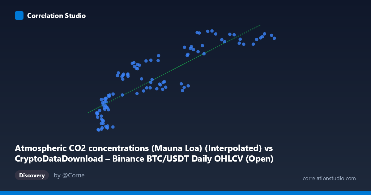
Atmospheric CO2 concentrations (Mauna Loa) (Interpolated) vs CryptoDataDownload – Binance BTC/USDT Daily OHLCV (Open)
- Pearson correlation (r)
- 0.8649
- Spearman correlation
- 0.8911
- p-value
- 0
- Sample size (n)
- 106
- 95% confidence interval
- 0.8073 to 0.9061
- Granger causality
- None
- Granger optimal lag
- 1
- Time coverage
- 2017-09-01 to 2026-06-01
- Recomputed on refreshed data
- 2026-10-08 (r was 0.8619)
AI analysis
Analysis: BTC/USDT Price vs. Atmospheric CO2 Concentration
1. What the Visualization Reveals
The scatterplot displays a strong positive association between Binance BTC/USDT price (X-axis, ranging from ~$3,434 to ~$115,764) and Mauna Loa atmospheric CO2 concentration (Y-axis, ranging from ~407 to ~428 ppm). As Bitcoin's price climbs across its historical range, CO2 readings rise in tandem, producing a curve that visually resembles a strong linear (or slightly concave) upward trend. The data points cluster into recognizable groups corresponding to Bitcoin's market cycles: a dense low-price cluster (~$3,400–$20,000, CO2 ~407–420 ppm) representing 2018–2020, and a sparser high-price cluster (~$60,000–$115,000, CO2 ~416–428 ppm) representing 2021–2025 bull runs.
2. Strength, Direction, and Statistical Meaning
The correlation coefficient (r = 0.862) indicates a strong positive linear relationship, with r² = 0.743 meaning roughly 74% of the variance in CO2 levels is statistically "explained" by BTC price movement. The 95% confidence interval [0.802, 0.905] is tight and does not cross zero, and the p-value of ~0 confirms this correlation is highly statistically significant — not due to random sampling noise. However, statistical significance here reflects the mathematical relationship, not a causal mechanism. Critically, the Granger causality tests show no significant predictive direction in either direction (X→Y: p=0.532; Y→X: p=0.736). This means neither variable's past values help forecast the other's future values — a strong indication that this is a spurious correlation driven by both series independently trending upward over the same calendar period (2017–2026), rather than any genuine causal or predictive link.
3. Notable Patterns and Features
The relationship is not perfectly linear — it shows a stepwise, cluster-like structure rather than smooth continuous covariation. Low-CO2/low-price points (2018–2020) form a tight band, while a middle cluster (~$27,000–$45,000, CO2 ~415–422 ppm) shows more scatter and even some inversions (e.g., $34,640 → 422.44 ppm vs. $43,820 → 417.14 ppm), suggesting the relationship weakens or reverses locally during Bitcoin's volatile consolidation phases. The high-price cluster ($90,000) shows CO2 plateauing near 426–428 ppm despite large BTC price swings, hinting at a ceiling effect — CO2's slow, steady annual rise cannot keep pace with Bitcoin's exponential volatility, causing the relationship to flatten at the extremes.
4. Confounding Factors and Caveats
This is a textbook case of confounding by shared time trend. Both atmospheric CO2 (rising steadily due to continuous fossil fuel emissions) and Bitcoin price (rising due to speculative demand, adoption, and market cycles) are non-stationary time series that trend upward over the 2017–2026 window. Any two upward-trending series will show high correlation regardless of causal connection — this is a well-known pitfall in time-series analysis. The lack of Granger causality strongly supports that the correlation is an artifact of co-trending rather than a meaningful economic or environmental relationship. Additionally, CO2 is measured monthly with very low variance (stdev = 6.36 ppm) while BTC price is daily and highly volatile (stdev = 31,870), so the two series operate on fundamentally different scales and dynamics.
5. Actionable Insights and Further Investigation
This correlation should not be used for forecasting or trading purposes — it has no predictive utility per the Granger results. To responsibly investigate any real relationship, analysts should: (a) detrend both series (e.g., differencing or using year-over-year changes) and retest correlation on the stationary residuals, which would likely collapse toward zero; (b) explicitly test for cointegration rather than raw correlation; and (c) if pursuing this comparison further, reframe it as a cautionary example of spurious correlation between unrelated non-stationary trends, useful for illustrating why r² and p-values alone are insufficient without causal/temporal validation like Granger tests.
X dataset: CryptoDataDownload – Binance BTC/USDT Daily OHLCV
Y dataset: Atmospheric CO2 concentrations (Mauna Loa)
Part of experiment: Bitcoin - CryptoDataDownload – Binance BTC/USDT Daily OHLCV vs Atmospheric CO2 concentrations (Mauna Loa)