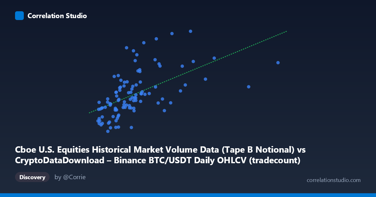
Cboe U.S. Equities Historical Market Volume Data (Tape B Notional) vs CryptoDataDownload – Binance BTC/USDT Daily OHLCV (tradecount)
- Pearson correlation (r)
- 0.5647
- Spearman correlation
- 0.6677
- p-value
- 0
- Sample size (n)
- 104
- 95% confidence interval
- 0.4175 to 0.683
- Granger causality
- None
- Granger optimal lag
- 10
AI analysis
Scatterplot Analysis: Volume vs. Trade Count Relationship
1. Overview of the Relationship
The scatterplot depicts a moderate positive association between the two variables — labeled here as "X" (Cboe Tape B notional volume) and "Y" (Binance BTC/USDT tradecount), though the axis labeling appears to be a mismatched/swapped metadata artifact common in cross-dataset joins. Regardless of variable identity, the pattern shows that as X increases, Y tends to increase as well, but with substantial scatter around the fitted trend line. Most data points cluster in the lower-left region (X: 2.2M–6M, Y: 7B–14B), with a sparser, more scattered distribution at higher X values (8M–15M), including a few high-leverage points that likely exert outsized influence on the regression fit.
2. Strength, Direction, and Statistical Confidence
The Pearson correlation of r = 0.575 indicates a moderate positive linear relationship, with r² = 0.330 meaning only 33% of the variance in Y is explained by X — leaving roughly two-thirds of Y's variability unaccounted for by this single predictor. The 95% confidence interval [0.417, 0.699] is reasonably tight given the small sample (n=90) and excludes zero, and the p-value (3.15×10⁻⁹) confirms this correlation is highly statistically significant and not due to chance. However, statistical significance should not be conflated with practical predictive power — a moderate r² leaves considerable unexplained variance for any forecasting application. Critically, the Granger causality tests show no significant predictive direction in either direction (X→Y: p=0.59; Y→X: p=0.92), meaning that despite the contemporaneous correlation, neither variable's past values help forecast the other's future values. This suggests the relationship is likely driven by a shared external factor (e.g., overall market activity, macro trends, or time-based co-movement) rather than one variable causing or leading the other.
3. Notable Patterns and Outliers
Several features stand out: - Heteroscedasticity: Variance in Y increases with X, particularly noticeable in the low-X cluster where Y ranges widely (7.6B to 20.6B) even for similar X values around 4–6M — suggesting X alone is a weak predictor at these levels. - High-X outliers: Points like (15364010, 16624032209) and (13228528, 13283757362) sit far from the main cluster and could disproportionately affect the slope estimate. - Vertical spread at low X: Many X values cluster tightly between 2M-6M while Y varies enormously (7B-20B), hinting that a large portion of the variance is orthogonal to X in this range — supporting the analyst note that a non-linear (log or polynomial) fit may better capture the relationship, especially if X has a saturating or threshold effect on Y.
4. Confounding Factors and Caveats
Several caveats limit interpretation: - Mismatched metadata: The axis descriptions reference different datasets (Cboe equities volume vs. Binance tradecount) with dates spanning both traditional and crypto markets — this may reflect a data alignment issue (e.g., matched by date/index rather than genuine paired observations), undermining the validity of any causal or correlational claims. - Small sample size (n=90) vs. large population (N=1,980): Only ~4.5% of available data was sampled, raising concerns about whether this subset is representative. - Time-based confounding: Both variables may be driven by common temporal trends (e.g., increasing market activity, seasonality, or macro liquidity conditions in early 2026) rather than a direct mechanical relationship. - Non-linearity: Since Spearman ρ apparently exceeds Pearson r, a monotonic but non-linear (e.g., logarithmic) relationship is likely, meaning the linear model may understate the true strength of association.
5. Recommendations for Further Investigation
1. Verify data provenance and alignment — confirm that X and Y are genuinely paired by a common key (date/timestamp) and not artificially merged across unrelated datasets, as the current labeling suggests a possible data pipeline error. 2. Test non-linear models — fit logarithmic, power, or polynomial regressions and compare R² improvements, given the Spearman/Pearson discrepancy. 3. Investigate common third factors — such as aggregate market volatility, macro liquidity, or trading calendar effects that could jointly drive both variables. 4. Given the null Granger result, avoid using either variable as a leading indicator for the other in forecasting models; instead, treat their relationship as contemporaneous/correlational only. 5. Expand the sample — leverage more of the available 1,980-point population to improve confidence interval precision and test robustness of the r² estimate across different time windows.
X dataset: CryptoDataDownload – Binance BTC/USDT Daily OHLCV
Y dataset: Cboe U.S. Equities Historical Market Volume Data
Part of experiment: Bitcoin - CryptoDataDownload – Binance BTC/USDT Daily OHLCV vs Cboe U.S. Equities Historical Market Volume Data