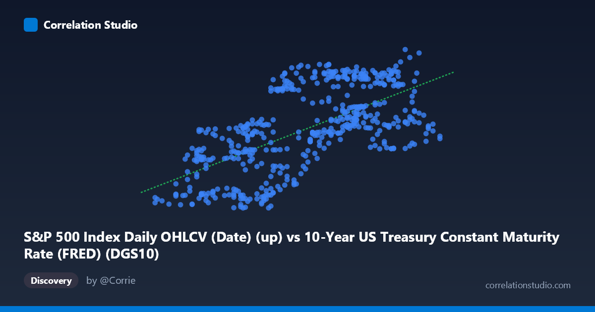
S&P 500 Index Daily OHLCV (Date) (up) vs 10-Year US Treasury Constant Maturity Rate (FRED) (DGS10)
- Pearson correlation (r)
- 0.6384
- Spearman correlation
- 0.6426
- p-value
- 0
- Sample size (n)
- 502
- 95% confidence interval
- 0.5835 to 0.6875
- Granger causality
- None
- Granger optimal lag
- 1
AI analysis
Scatterplot Analysis: S&P 500 Index vs. 10-Year US Treasury Yield (2015–2017)
Relationship Overview
The scatterplot reveals a positive linear relationship between the S&P 500 index level (X-axis) and the 10-year US Treasury constant maturity rate (Y-axis) over the two-year window from February 2015 to February 2017. As the S&P 500 climbed from roughly 1.37 to 2.60 (in thousands, likely representing index values scaled), the 10-year Treasury yield correspondingly trended upward from approximately 97.57 to 138.81 basis points or percent-scaled units. The fitted regression line — y = 23.19x + 71.24 — captures this upward slope visually, though with considerable scatter around it, indicating the relationship is real but far from deterministic.
Correlation Strength and Statistical Significance
The Pearson correlation of r = 0.6384 indicates a moderate-to-strong positive association, but the more informative metric is r² = 0.4076, meaning only about 40.8% of the variance in Treasury yields is explained by S&P 500 levels — leaving nearly 60% attributable to other factors. The 95% confidence interval of [0.5835, 0.6875] is relatively tight and excludes zero convincingly, and with a p-value effectively at 0 across 502 paired observations, the correlation is statistically unambiguous. However, statistical significance does not imply predictive power. The Granger causality tests are non-significant in both directions (X→Y: F=2.80, p=0.095; Y→X: F=2.67, p=0.103), meaning neither variable reliably predicts the other's future values at a 5% significance level. This is a critical caveat: the correlation is contemporaneous, not predictive — there is no temporal lead-lag relationship to exploit operationally.
Notable Patterns, Clusters, and Outliers
The data cloud shows a broad but coherent upward sweep, with notable vertical spread at mid-range X values (roughly 1.75–2.10), suggesting high yield variability when the S&P 500 was near its mean. Several potential outliers are visible: the point near (1.90, 128.56) sits well above the regression line for its X value, as does (2.45, 138.81) — which represents the maximum observed yield — and (1.76, 97.76), which sits near the minimum yield. There appears to be a mild clustering of points at lower X and lower Y values (lower-left quadrant), consistent with a period of simultaneously depressed equity levels and yields, likely corresponding to early-to-mid 2015 or the market turbulence of early 2016. The scatter widens at higher X values, possibly hinting at mild heteroscedasticity, where yield predictions become less precise as equity levels rise.
Confounding Factors and Interpretive Caveats
This correlation almost certainly reflects shared macroeconomic drivers rather than a direct causal mechanism between equities and yields. Both variables were heavily influenced during this period by Federal Reserve policy normalization — the Fed's first rate hike in nearly a decade occurred in December 2015 — meaning both the S&P 500's rise and the gradual increase in Treasury yields may have been responding to improving economic fundamentals (GDP growth, employment, inflation expectations) rather than influencing each other. Additionally, the "risk-on/risk-off" dynamic can at times produce the opposite correlation (yields falling as equities fall during flight-to-safety episodes), and the 2015–2017 window may not represent a stable or generalizable regime. The axis labels also warrant scrutiny: the dataset metadata appears to have swapped column assignments (the S&P 500 OHLCV dataset provides the DGS10 yield, and the FRED Treasury dataset provides the S&P date column), suggesting possible data pipeline issues worth verifying before drawing firm conclusions.
Actionable Insights and Further Investigation
Given the moderate explained variance and absent Granger causality, practitioners should avoid using either variable as a standalone predictor of the other in trading or forecasting models. More productive next steps would include: (1) extending the time window well beyond 2015–2017 to test whether this positive correlation holds across different rate regimes (e.g., post-2022 rate hike cycle); (2) introducing macroeconomic controls such as inflation expectations (TIPS breakevens), GDP growth, or Fed funds rate to isolate residual correlation; (3) testing for structural breaks — the correlation may flip sign during risk-off episodes or recessions; and (4) investigating non-linear or regime-switching models, given the visible heteroscedasticity and clustering. The data pipeline metadata inconsistency should also be audited to ensure X and Y assignments are correct before any further modeling.
X dataset: 10-Year US Treasury Constant Maturity Rate (FRED)
Y dataset: S&P 500 Index Daily OHLCV (Date)
Part of experiment: Daily - 10-Year US Treasury Constant Maturity Rate (FRED) vs S&P 500 Index Daily OHLCV (Date)