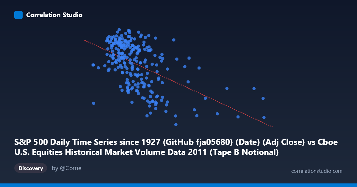
S&P 500 Daily Time Series since 1927 (GitHub fja05680) (Date) (Adj Close) vs Cboe U.S. Equities Historical Market Volume Data 2011 (Tape B Notional)

Pearson correlation (r): -0.5247
Spearman correlation: -0.4926
p-value: 0
Sample size (n): 252
95% confidence interval: -0.6088 to -0.4289
Granger causality: X → Y
Granger optimal lag: 10

AI analysis

Analysis: S&P 500 Adjusted Close Price vs. Cboe Tape B Notional Volume (2011)

Relationship Overview

The scatterplot reveals a moderate negative relationship between the S&P 500 adjusted closing price (X-axis) and Cboe Tape B notional trading volume (Y-axis) across 252 trading days in 2011. As the S&P 500 price level increases, Tape B notional volume tends to decrease, and conversely, lower price levels are associated with higher notional volume. This inverse pattern is visually evident as a downward-sloping cloud of points, consistent with the fitted linear regression: y = -1.827×10⁻⁸x + 1361.04. The relationship makes intuitive sense in the context of 2011 market dynamics, a year characterized by the European sovereign debt crisis, U.S. debt ceiling debates, and significant equity market volatility — periods of market stress (lower S&P levels) often coincide with elevated trading activity as investors reposition defensively.

Correlation Strength and Statistical Significance

The Pearson correlation of r = -0.5247 indicates a moderate negative association, but the explanatory power is more sobering when expressed through R²: only 27.5% of the variance in Tape B notional volume is explained by the S&P 500 price level, leaving nearly three-quarters of variation attributable to other factors. The 95% confidence interval of [-0.6088, -0.4289] is entirely negative and reasonably tight, confirming the direction of the relationship with good confidence. With a p-value of effectively zero and a sample of n = 252 drawn from a population of N = 3,780, the result is highly statistically significant — this is not a chance finding. The Granger causality analysis adds a critical temporal dimension: X (S&P 500 price) Granger-causes Y (Tape B notional volume) unidirectionally at an optimal lag of 10 trading periods (approximately two calendar weeks), with F = 1.8777 (p = 0.0494). The reverse direction fails to reach significance (F = 0.4151, p = 0.9385). This suggests that S&P 500 price movements have modest but statistically meaningful predictive utility for Tape B volume roughly two weeks later, while volume does not predict price in this dataset — an asymmetry worth noting for market microstructure analysis.

Notable Patterns, Clusters, and Outliers

Several structural features stand out in the data. There is a dense cluster of points concentrated between approximately 3.0–6.0 billion on the X-axis and 1,240–1,360 on the Y-axis, reflecting the majority of 2011 trading days when the S&P 500 hovered in a mid-range band. However, a notable right-tail scatter extends toward X values of 8–14 billion, corresponding to unusually high S&P 500 price readings; these points consistently show lower Tape B notional values (around 1,130–1,290), reinforcing the negative trend. Several potential outliers are visible at extreme Y values — points near 1,100 paired with mid-range X values that deviate substantially from the regression line — which may correspond to specific high-stress trading sessions or exchange-specific anomalies. The spread of residuals also appears to widen at lower X values (heteroscedasticity), suggesting the relationship is less predictable when the S&P 500 is at depressed levels, precisely when market behavior is most chaotic.

Confounding Factors and Interpretive Caveats

Several important caveats temper interpretation. First, Tape B specifically covers NYSE American (AMEX) and regional exchange listings, not the full market, so this notional figure reflects a subset of trading activity that may be disproportionately influenced by small- and mid-cap stock behavior rather than the broad market. Second, notional volume is price-sensitive by construction — if the securities comprising Tape B themselves track broader market prices, some of the observed negative correlation could be a mechanical artifact rather than a behavioral signal. Third, 2011 was a structurally unusual year with two discrete volatility regimes (relative calm in H1, sharp correction and recovery in H2), which could be artificially inflating the correlation by creating a bimodal distribution masquerading as a linear trend. Finally, the Granger causality result, while statistically significant, sits right at the p = 0.05 threshold (p = 0.0494), warranting caution against over-interpreting predictive directionality without out-of-sample validation.

Actionable Insights and Further Investigation

For practitioners, the 10-period Granger lag suggests that sustained S&P 500 price declines may serve as a leading indicator of elevated Tape B volume approximately two weeks hence, which could be useful for exchange capacity planning or liquidity provision strategies. However, given that R² explains only 27.5% of variance, building any operational model on this relationship alone would be insufficient. Recommended next steps include: (1) segmenting the analysis by market regime (pre/post August 2011 correction) to test whether the correlation is driven primarily by one period; (2) incorporating VIX or implied volatility as a co-variate to isolate behavioral volume responses from price-mechanical effects; (3) testing the same relationship on Tape A and Tape C to determine whether this is a Tape B–specific phenomenon or market-wide; and (4) extending the dataset beyond 2011 to assess whether the Granger causal structure is stable across different market environments or is a feature specific to crisis-period dynamics.

X dataset: Cboe U.S. Equities Historical Market Volume Data 2011

Y dataset: S&P 500 Daily Time Series since 1927 (GitHub fja05680) (Date)

Part of experiment: Daily - Cboe U.S. Equities Historical Market Volume Data 2011 vs S&P 500 Daily Time Series since 1927 (GitHub fja05680) (Date)