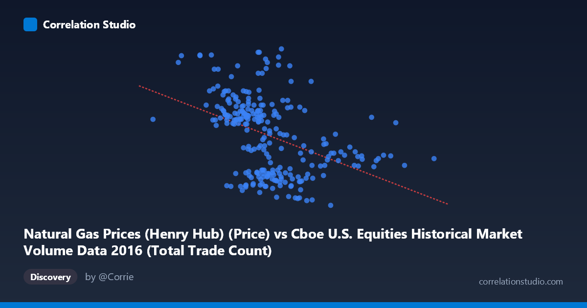
Natural Gas Prices (Henry Hub) (Price) vs Cboe U.S. Equities Historical Market Volume Data 2016 (Total Trade Count)
- Pearson correlation (r)
- -0.4196
- Spearman correlation
- -0.4624
- p-value
- 0
- Sample size (n)
- 252
- 95% confidence interval
- -0.5164 to -0.3123
- Granger causality
- None
- Granger optimal lag
- 1
AI analysis
Scatterplot Analysis: Natural Gas Prices vs. Cboe Equity Trade Count (2016)
Relationship Overview The scatterplot reveals a modest negative relationship between Henry Hub natural gas spot prices (X-axis) and Cboe U.S. equity market total trade counts (Y-axis) across 2016. As natural gas prices increase, trade counts tend to decline slightly, following the regression line y = -4.45278E⁻⁷x + 3.596. The data cloud is broadly dispersed, suggesting the linear trend exists but explains only a fraction of the variability in trade counts. Most observations cluster in the natural gas price range of roughly $1.75–$3.50, with trade counts concentrated between approximately 2.0 and 3.0 (likely in millions), indicating that extreme values in either direction are relatively rare.
Correlation Strength and Statistical Significance The Pearson correlation of r = -0.4196 indicates a weak-to-moderate negative association. However, r² = 0.176 means that natural gas prices explain only 17.6% of the variance in equity trade counts — leaving over 82% attributable to other factors. While the 95% confidence interval of [-0.516, -0.312] confirms the direction is reliably negative and does not cross zero, the width of this interval reflects meaningful uncertainty about the true population effect size. The p-value of 3.6E-12 confirms the correlation is highly statistically significant, which is unsurprising given the large population size (N = 3,622); statistical significance here should not be conflated with practical or economic significance. Critically, Granger causality tests find no significant predictive relationship in either direction (X→Y: F = 0.83, p = 0.363; Y→X: F = 0.34, p = 0.563), meaning neither variable temporally predicts the other at a one-period lag. This substantially weakens any causal narrative between the two series.
Notable Patterns, Clusters, and Outliers The bulk of the data clusters between natural gas prices of $1.8M–$2.8M (in the price unit shown) and trade counts of 2.0–3.1, forming a dense elliptical cloud consistent with the moderate correlation. Several notable outliers are visible: a small group of high trade-count observations (~3.5–3.8) occurring at relatively low natural gas prices (~1.6M–2.0M range), including the point near (1,722,715, 3.50) and (2,538,868, 3.56), which may correspond to high-volatility equity trading sessions. At the upper end of natural gas prices (above ~3.2M), trade counts appear compressed into a narrower range (~2.1–2.3), suggesting a potential ceiling effect or simply fewer extreme equity market events during high gas-price periods. There is no strong evidence of a non-linear pattern, but the scatter fan appears slightly wider at lower gas prices, hinting at mild heteroscedasticity.
Confounding Factors and Caveats The apparent correlation likely reflects shared seasonality rather than any direct causal mechanism. Both natural gas prices and equity trading volumes exhibit seasonal patterns — gas prices tend to be lower in summer and higher in winter, while equity volumes are influenced by earnings cycles, macroeconomic announcements, and end-of-year effects. Any co-movement between them across 2016 could easily be driven by a common temporal trend (e.g., January and February 2016 saw significant market volatility coinciding with a gas price environment) rather than a structural relationship. Additionally, the dataset covers only a single calendar year (2016), limiting generalizability. The axis labels appear inverted in the dataset descriptions (prices are on X, trade counts on Y), and care should be taken to verify unit consistency, as the X-axis values in the millions suggest these may be index-scaled or volume-adjusted figures rather than raw dollar prices.
Actionable Insights and Further Investigation Given the absence of Granger causality and the low explained variance, these variables should not be used as predictors of one another in a trading or forecasting model without substantial additional evidence. However, the correlation warrants deeper investigation into whether a common latent driver — such as macroeconomic uncertainty indices (VIX), Federal Reserve policy announcements, or seasonal demand cycles — simultaneously influences both series. Researchers should consider: (1) extending the analysis to multiple years to test whether the negative correlation is consistent or an artifact of 2016 conditions; (2) applying seasonal decomposition (e.g., STL decomposition) to remove shared seasonal trends before re-testing the correlation; (3) testing longer Granger lags (beyond 1 period) and incorporating multivariate models with control variables. If the correlation persists after deseasonalization, it could reflect a genuine cross-market risk-appetite signal worth further exploration.
X dataset: Cboe U.S. Equities Historical Market Volume Data 2016
Y dataset: Natural Gas Prices (Henry Hub)
Part of experiment: Daily - Cboe U.S. Equities Historical Market Volume Data 2016 vs Natural Gas Prices (Henry Hub)