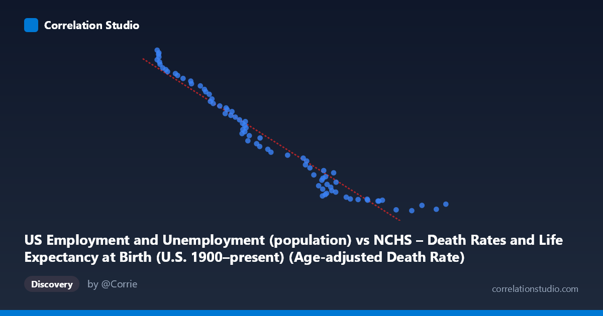
US Employment and Unemployment (population) vs NCHS – Death Rates and Life Expectancy at Birth (U.S. 1900–present) (Age-adjusted Death Rate)
- Pearson correlation (r)
- -0.972
- Spearman correlation
- -0.99
- p-value
- 0
- Sample size (n)
- 78
- 95% confidence interval
- -0.9821 to -0.9563
- Granger causality
- None
- Granger optimal lag
- 10
- Time coverage
- 1941-01-01 to 2018-01-01
AI analysis
Analysis: U.S. Employment Population vs. Age-Adjusted Death Rate (1941–2018)
1. Overall Relationship The scatterplot reveals a strong, consistent negative relationship between the U.S. employment/unemployment population size and the age-adjusted death rate. As the employment population metric (X) increases over time — broadly reflecting a growing and economically active labor force — the age-adjusted death rate (Y) declines substantially, from values exceeding 250,000 down toward approximately 93,000–100,000. The data points follow a tight, nearly linear downward trajectory across the full range, suggesting these two long-run time series move in close opposition across the 77-year observation window.
2. Correlation Strength and Statistical Framing The Pearson correlation of r = −0.972 is exceptionally strong, and the R² of 0.9447 means that roughly 94.5% of the variance in age-adjusted death rates is statistically explained by variation in the employment population measure. The 95% confidence interval of [−0.9821, −0.9563] is narrow and entirely negative, confirming this is not a sampling artifact, and the p-value of effectively zero eliminates any reasonable doubt about statistical significance. However, the Granger causality results tell a critically different story: neither direction (X→Y nor Y→X) achieves significance at the optimal 10-period lag (F = 1.657, p = 0.120 and F = 1.540, p = 0.155, respectively). This means that despite the extraordinary correlational strength, neither variable temporally predicts the other beyond what each already predicts from its own past values. This is a decisive caution against any causal interpretation.
3. Patterns, Clusters, and Notable Features The scatterplot exhibits several visually distinct features. At the high-Y, low-X end (roughly X < 850, Y 235,000), a small but tight cluster of points appears, corresponding to the earliest years of the dataset (early-to-mid 1940s) when both the labor force was smaller and death rates were higher. At the opposite extreme (X 1,600, Y < 110,000), another cluster of more recent observations forms, again tightly grouped. The middle range (X: 900–1,400; Y: 110,000–230,000) is densely populated and follows the linear trend with very little scatter. A few points — notably around (1,830, 99,900), (1,705, 93,220), and (776, 257,791) — sit at the extremes of both axes but remain on-trend rather than being true outliers, confirming the robustness of the linear fit. No pronounced non-linearity is visually apparent, though there is a subtle suggestion of slight curvature at the lower-X end.
4. Confounding Factors and Interpretive Caveats The most important caveat is that both variables are proxies for the passage of time. Over 1941–2018, the U.S. employment population grew steadily due to population growth, demographic expansion, and women's labor force entry, while age-adjusted death rates declined due to medical advances, public health improvements, reduced smoking, and better nutrition. These are both secular trends driven by modernization, not causally linked phenomena. The near-perfect correlation is therefore a classic case of spurious correlation via shared time trend — a well-known statistical hazard with long time-series data. The Granger non-causality result is consistent with this interpretation. Additionally, the employment population figure likely reflects total population growth as much as labor market conditions, and "age-adjusted death rate" aggregates across vastly different causes of death that have distinct determinants.
5. Actionable Insights and Further Investigation Rather than treating this correlation as meaningful on its own, analysts should detrend both series (e.g., by differencing or including a time trend variable) to determine whether any residual relationship exists after removing the shared temporal component. It would be valuable to disaggregate by cause of death (cardiovascular, infectious disease, cancer) and examine whether specific employment-related factors — occupational safety, income, healthcare access — correlate with specific mortality subcategories after controlling for time. Regime-change analysis (e.g., structural breaks around recessions, the 2008 financial crisis, or major public health events) could reveal whether the relationship holds uniformly or only during particular economic periods. Finally, incorporating lagged GDP, healthcare expenditure, or poverty rates as covariates would help isolate whether any employment-mortality linkage survives multivariate controls — transforming a striking but likely spurious bivariate finding into a potentially actionable causal model.
X dataset: NCHS – Death Rates and Life Expectancy at Birth (U.S. 1900–present)
Y dataset: US Employment and Unemployment
Part of experiment: Yearly - NCHS – Death Rates and Life Expectancy at Birth (U.S. 1900–present) vs US Employment and Unemployment