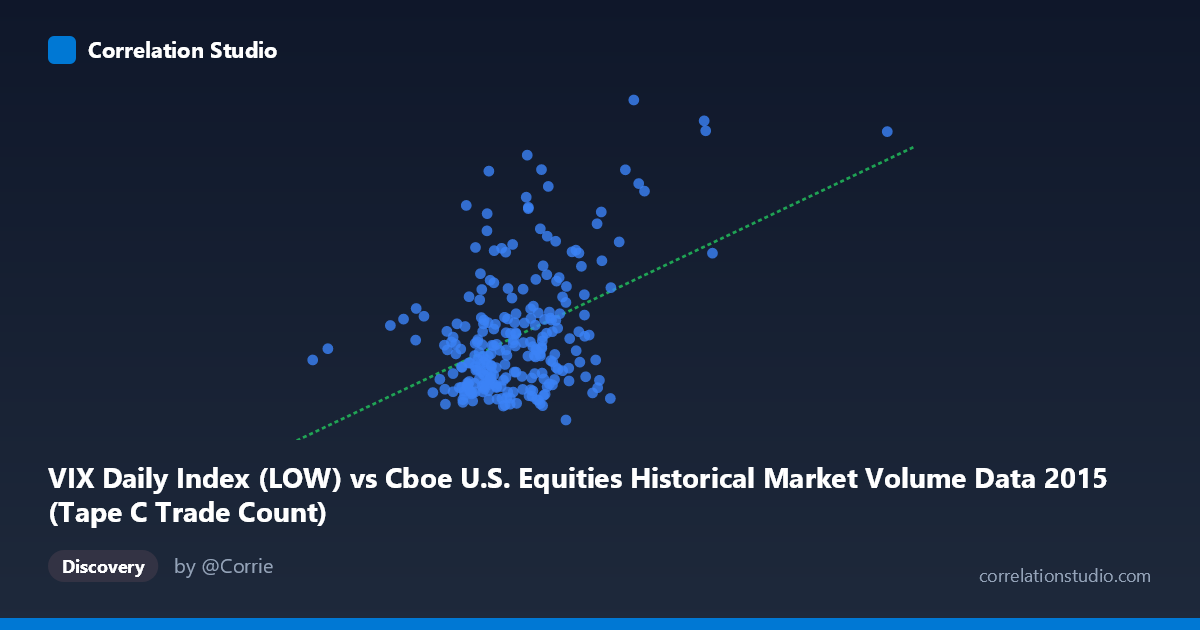
VIX Daily Index (LOW) vs Cboe U.S. Equities Historical Market Volume Data 2015 (Tape C Trade Count)
- Pearson correlation (r)
- 0.4444
- Spearman correlation
- 0.2881
- p-value
- 0
- Sample size (n)
- 252
- 95% confidence interval
- 0.3394 to 0.5384
- Granger causality
- None
- Granger optimal lag
- 1
AI analysis
Scatterplot Analysis: VIX Low vs. Tape C Trade Count (2015)
Overall Relationship The scatterplot reveals a moderate positive relationship between the Cboe VIX Daily Low index and the Tape C Trade Count for U.S. equities in 2015. As the VIX low value increases — indicating elevated baseline volatility — the number of Tape C trades tends to rise as well. This is intuitively consistent with market microstructure theory: higher volatility environments typically attract greater trading activity as market participants respond to price uncertainty, hedge positions, or seek arbitrage opportunities. The linear regression equation (y = 1.23086E-05x + 6.52403) confirms a positive slope, though the relationship is far from deterministic, with considerable vertical scatter visible throughout the distribution.
Correlation Strength and Statistical Significance The Pearson correlation of r = 0.444 indicates a moderate positive association, but the explanatory power is limited: r² = 0.197 means that only 19.7% of the variance in Tape C Trade Count is explained by the VIX Low. The remaining ~80% is attributable to other factors entirely. The 95% confidence interval for r of [0.339, 0.538] is meaningfully above zero, and the p-value of 1.277E-13 confirms the relationship is highly statistically significant given the population of N = 3,302 and paired sample of n = 252. However, statistical significance here should not be conflated with practical magnitude — the effect size is real but modest. Critically, the Granger causality tests show no significant directional predictive relationship in either direction (X→Y: F = 0.13, p = 0.716; Y→X: F = 0.02, p = 0.889), meaning neither variable reliably predicts the other's future values at a one-period lag. This rules out straightforward temporal forecasting applications.
Notable Patterns and Outliers Several features stand out in the sample data. There is a visible cluster of points concentrated in the X range of roughly 600,000–900,000 and Y range of 11–18, representing the typical trading-day regime. Above this core cluster, a secondary grouping emerges at higher VIX lows (roughly 900,000–1,200,000+), associated with elevated trade counts (20–29), likely corresponding to volatility episodes such as the August 2015 market correction. Points like (1,194,527, 28.08) and (1,040,483, 24.94) appear as notable high-leverage outliers that may be disproportionately influencing the regression slope. On the lower end, (291,078, 14.45) stands as an extreme X-axis outlier with a comparatively unremarkable Y value, suggesting a day of anomalously low market volume that did not coincide with unusual volatility.
Confounding Factors and Caveats Several important caveats apply. First, the axis assignment appears counterintuitive: the VIX Low (a volatility index measure) is plotted on the X-axis with values in the hundreds of thousands, while Tape C Trade Count (raw trade counts) appears on the Y-axis with values in the 10–30 range — these scales suggest possible unit inconsistencies or dataset labeling mismatches that warrant verification. Second, both variables are likely driven by common macro-level confounders such as Federal Reserve announcements, earnings seasons, geopolitical events, and index rebalancing days, which could create spurious correlation without a direct causal mechanism. Third, the data covers only calendar year 2015, a period that included a notable volatility spike; results may not generalize to other years.
Actionable Insights and Further Investigation Given the moderate correlation and absent Granger causality, the VIX Low alone is insufficient as a standalone predictor of Tape C trading activity. Recommended next steps include: (1) conducting a multivariate regression incorporating VIX High, VIX Close, and total market volume to better isolate the VIX Low's marginal contribution; (2) examining the relationship during the August 2015 volatility event specifically as a sub-period analysis to determine whether the correlation strengthens in stress regimes; (3) testing non-linear models (e.g., polynomial or threshold regression) given the apparent heteroscedasticity — variance in trade counts appears to expand at higher VIX levels; and (4) verifying the dataset column alignment, as the axis labels suggest the X and Y variable sources may have been transposed during data merging.
X dataset: Cboe U.S. Equities Historical Market Volume Data 2015
Y dataset: VIX Daily Index
Part of experiment: Daily - Cboe U.S. Equities Historical Market Volume Data 2015 vs VIX Daily Index