NOAA ISD Weather Station History (Lat/Lon Index) (STP_ATTRIBUTES) vs CryptoDataDownload – Binance BTC/USDT Daily OHLCV (Low)
- Pearson correlation (r)
- -0.4768
- Spearman correlation
- -0.3268
- p-value
- 0
- Sample size (n)
- 355
- 95% confidence interval
- -0.5534 to -0.3921
- Granger causality
- None
- Granger optimal lag
- 1
AI analysis
Analysis of Variable Relationship
1. Overview of the Visualization
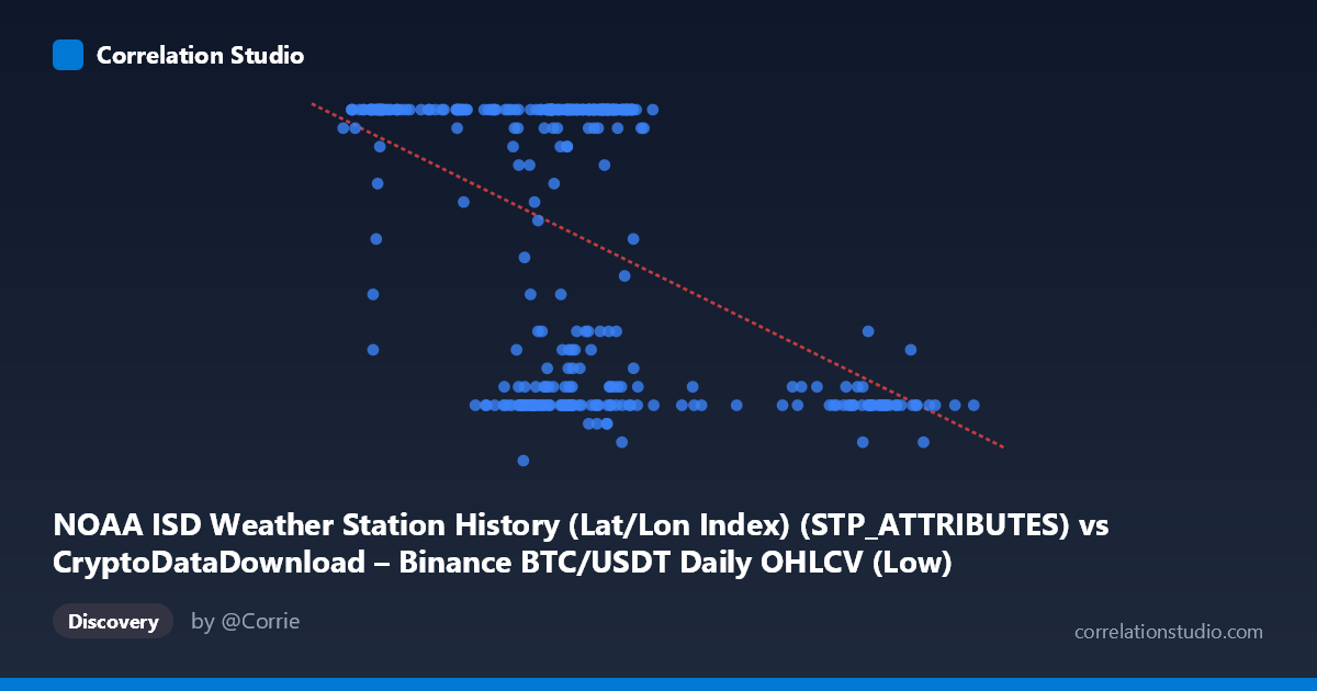
The scatterplot shows a moderate negative relationship between the X variable (labeled as a weather station index, though the values—ranging ~38,555 to 105,321—more plausibly represent something like a price or timestamp-derived metric) and Y (ranging 5–24, with a suspicious ceiling effect at exactly 24). The data shows a dense cluster of points between X≈40,000–70,000, with a sparser tail extending to ~105,000. Notably, Y=24 appears with high frequency across a wide span of X values (roughly 41,000–70,000), suggesting this may be a capped or censored value rather than a naturally continuous measurement.
2. Strength, Direction, and Statistical Confidence
The correlation coefficient of r = -0.4768 indicates a moderate negative linear relationship: as X increases, Y tends to decrease. However, r² = 0.2273 means only about 22.7% of the variance in Y is explained by X—the majority (77%) of Y's variability is driven by other factors not captured here. The 95% confidence interval [-0.5534, -0.3921] is reasonably tight and does not cross zero, and the p-value of ~0 confirms this correlation is statistically significant and not due to chance, given N=355.
Importantly, the Granger causality test shows no significant predictive direction in either direction (X→Y: p=0.66; Y→X: p=0.26). This means that despite the contemporaneous correlation, neither variable helps forecast the other over time using lagged values. This is a critical distinction: correlation here reflects a static/contemporaneous association, not a temporal lead-lag relationship. This finding also casts doubt on treating this as a meaningful causal or predictive pairing.
3. Notable Patterns and Anomalies
Several structural features stand out: - Ceiling/saturation at Y=24: A large proportion of points sit exactly at Y=24 across diverse X values, suggesting a cap, categorical binning, or data artifact rather than continuous variation. - Bimodal-like clustering: Points seem to split into a "high Y" group (mostly Y=22–24) concentrated at lower-to-mid X (40,000–70,000) and a "low Y" group (Y=7–12) appearing both in the mid-X range and at higher X values (85,000–105,000). - Sparse high-X tail: Beyond X=85,000, only low Y values (8–11) appear, pulling the regression line downward and likely inflating the apparent negative correlation. - The regression line (y = -0.000254x + 33.27) is heavily influenced by this sparse tail; without it, the relationship in the dense cluster may be weaker or noisier.
4. Confounding Factors and Caveats
The metadata is confusing and likely mismatched: X is labeled as a NOAA weather station attribute, but its range and description align with financial data (BTC/USDT OHLCV), while Y is labeled as "Low" price but only takes integer values 5–24, more consistent with a weather-related count (e.g., wind speed, cloud cover code, or day count) than a crypto price. This suggests column mislabeling or a data-merging error, which should be resolved before drawing substantive conclusions. Additionally, the Y=24 ceiling suggests possible data truncation, categorical encoding, or a missing-value placeholder—any of which would distort the correlation and r² estimate.
5. Suggested Next Steps
1. Verify data provenance and labels—confirm whether X and Y are correctly matched to their described sources, as the current labels appear inconsistent with the value ranges. 2. Investigate the Y=24 cluster—determine if this is a true ceiling, a default/missing-value code, or a legitimate mode, and consider re-running correlation after excluding or separately modeling these points. 3. Segment the analysis by the apparent X clusters (e.g., <70,000 vs. 85,000) to check if the negative correlation is driven mainly by the sparse high-X tail rather than a consistent trend. 4. Given the null Granger causality result, avoid using this relationship for forecasting; instead, treat it as descriptive/contemporaneous only, and explore other lag structures or non-linear time-series models if temporal prediction is the goal. 5. Consider non-linear or categorical modeling (e.g., logistic/ordinal regression) given the discrete, bounded nature of Y, which may not be well-served by simple linear regression despite the reported R².
X dataset: CryptoDataDownload – Binance BTC/USDT Daily OHLCV
Y dataset: NOAA ISD Weather Station History (Lat/Lon Index)
Part of experiment: Bitcoin - CryptoDataDownload – Binance BTC/USDT Daily OHLCV vs NOAA ISD Weather Station History (Lat/Lon Index)