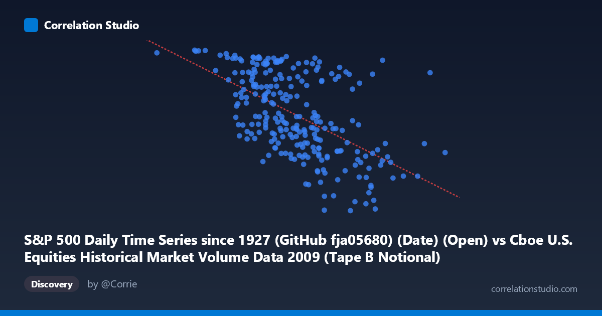
S&P 500 Daily Time Series since 1927 (GitHub fja05680) (Date) (Open) vs Cboe U.S. Equities Historical Market Volume Data 2009 (Tape B Notional)
- Pearson correlation (r)
- -0.564
- Spearman correlation
- -0.5779
- p-value
- 0
- Sample size (n)
- 252
- 95% confidence interval
- -0.6428 to -0.4735
- Granger causality
- Bidirectional
- Granger optimal lag
- 10
AI analysis
Analysis: S&P 500 Open Price vs. Cboe Tape B Notional Volume (2009)
Relationship Overview The scatterplot reveals a moderate negative relationship between S&P 500 daily open prices (X-axis, measured as Unix timestamps representing dates in 2009) and Cboe Tape B notional trading volume (Y-axis). As the year progresses — from the market lows of early 2009 through the recovery — Tape B notional volume tends to decline. This is visually intuitive: the extreme fear and volatility of early 2009 (post-financial crisis) drove elevated trading activity, while the gradual market stabilization later in the year corresponded with reduced notional volume on smaller-cap exchanges. The linear regression equation y = -4.97e-08x + 1209.1 captures this downward trajectory, though the scatter around the line is considerable.
Correlation Strength and Statistical Significance The Pearson correlation of r = -0.564 indicates a moderate negative association, with r² = 0.318 meaning that only 31.8% of the variance in Tape B notional volume is explained by the date/price progression — leaving nearly 70% attributable to other factors. The 95% confidence interval of [-0.643, -0.474] is meaningfully narrow given n = 252 paired observations from a population of N = 3,232, and the p-value of effectively zero confirms this relationship is not a statistical artifact. Granger causality tests reveal bidirectional temporal predictive relationships at an optimal lag of 10 trading periods: X→Y (F = 2.01, p = 0.033) and Y→X (F = 1.93, p = 0.042). Both directions are statistically significant but with modest F-statistics, suggesting weak mutual predictability rather than a dominant causal arrow — neither variable strongly "leads" the other.
Notable Patterns and Outliers Several features stand out in the sample points. The early-year observations (timestamps near 1.32 billion, e.g., January 2009) cluster at high Y values (~1,121), consistent with peak crisis-era volume. Conversely, mid-to-late year points scatter more widely, with several low-volume outliers visible — notably (6,821,195,810, 679.28) and (7,526,902,255, 684.04), suggesting specific late-year sessions with anomalously suppressed Tape B activity. The spread of Y values (679–1,129) is substantial across all X ranges, indicating high intra-period variance that the linear model cannot fully capture. There is also a hint of a non-linear "funnel" pattern where variance in Y appears larger at earlier timestamps and compresses somewhat later, potentially indicating heteroscedasticity.
Confounding Factors and Caveats Several important caveats apply. First, the X-axis encodes time as a Unix timestamp, meaning this correlation is fundamentally a time-series trend analysis rather than a direct causal price-volume relationship — both variables are co-evolving with the post-crisis recovery narrative. Seasonality, Federal Reserve interventions, quarterly earnings cycles, and index rebalancing events could all drive volume patterns independently. Second, Tape B specifically covers NYSE American (AMEX) and regional exchange stocks, which may respond differently to macro conditions than broad market volume. Third, the bidirectional Granger causality with modest F-statistics warrants caution — statistical significance at n = 252 does not imply economic meaningfulness, and the 10-period lag structure may be capturing shared macro rhythms rather than genuine predictive signal.
Actionable Insights and Further Investigation Practitioners should decompose the time trend by regressing out the temporal component and examining the residual price-volume relationship. It would be valuable to compare Tape B with Tape A (NYSE) and Tape C (Nasdaq) volumes to determine whether the pattern is exchange-specific or market-wide. Volatility indices (VIX) should be introduced as a mediating variable, as volatility likely explains much of the early-2009 volume spike independently of price level. Given the bidirectional Granger result, a Vector Autoregression (VAR) model at 10-period lags could better quantify the feedback dynamics. Finally, replicating this analysis across other crisis and recovery years (2008, 2020) would test whether this negative date-volume relationship is a generalizable crisis-recovery signature or specific to 2009 market microstructure conditions.
X dataset: Cboe U.S. Equities Historical Market Volume Data 2009
Y dataset: S&P 500 Daily Time Series since 1927 (GitHub fja05680) (Date)
Part of experiment: Daily - Cboe U.S. Equities Historical Market Volume Data 2009 vs S&P 500 Daily Time Series since 1927 (GitHub fja05680) (Date)