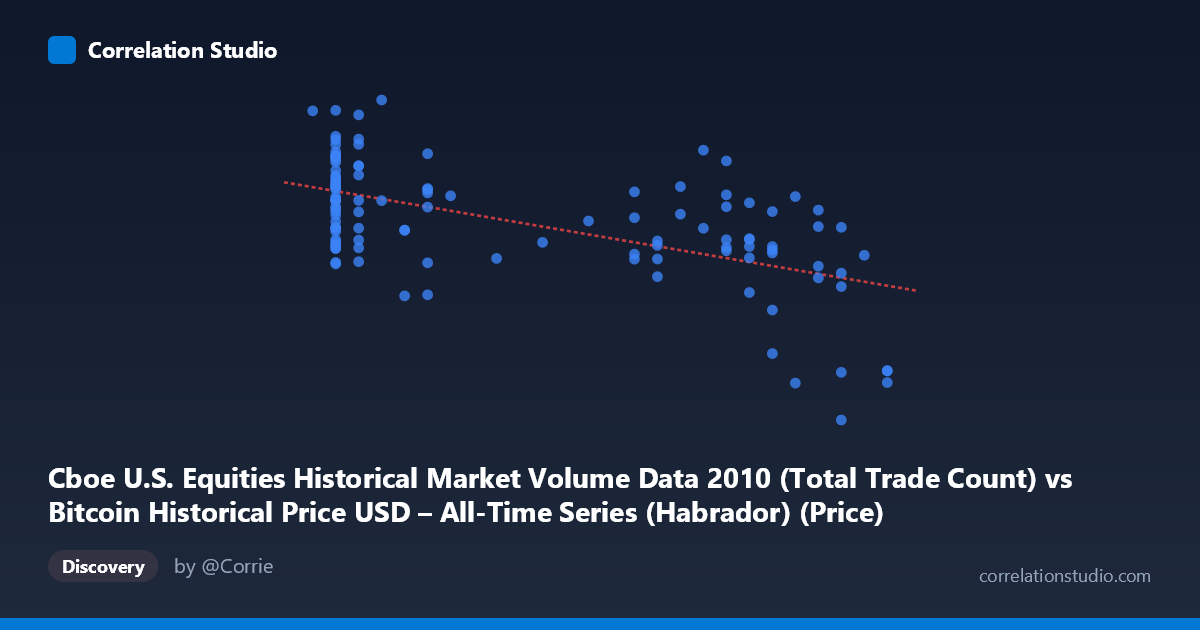
Cboe U.S. Equities Historical Market Volume Data 2010 (Total Trade Count) vs Bitcoin Historical Price USD – All-Time Series (Habrador) (Price)
- Pearson correlation (r)
- -0.5852
- Spearman correlation
- -0.5235
- p-value
- 0
- Sample size (n)
- 117
- 95% confidence interval
- -0.6931 to -0.4516
- Granger causality
- None
- Granger optimal lag
- 10
AI analysis
Analysis: Trade Count vs. Bitcoin Price (2010)
1. What the Visualization Reveals
The scatterplot shows a moderate negative relationship between Cboe U.S. equities trade count and Bitcoin's historical price. As the X-axis variable increases from roughly 0.05 to 0.30, Y-values (Bitcoin price) trend downward from a cluster near $1.8–2.5M down toward $650K–950K at the highest X values. However, the relationship is clearly noisy rather than a clean linear decline — there's substantial vertical scatter at every X value, particularly in the 0.06–0.10 range where Y-values span from ~1.39M to ~2.57M.
2. Strength, Direction, and Uncertainty
The correlation coefficient (r = -0.585) indicates a moderate negative linear relationship, with r² = 0.342 meaning only 34% of the variance in Y is explained by X — leaving 66% unexplained by this linear model alone. The 95% CI [-0.693, -0.452] is reasonably tight and entirely negative, and the p-value (4.25E-12) is highly significant, giving strong confidence that a real negative association exists in this sample — this is not a chance finding. However, statistical significance should not be conflated with practical predictive power: a relationship explaining only one-third of variance leaves considerable room for error in any point prediction. Critically, the Granger causality tests (p = 0.77 and p = 0.62 in both directions) show no evidence of temporal predictive causality either way, meaning past values of one series do not meaningfully help forecast the other — the correlation is contemporaneous/associational only, not causal or predictive in a time-series sense.
3. Notable Patterns and Outliers
The data shows distinct clustering rather than a smooth continuum: a dense cluster at low X (0.06–0.10) with high, widely-scattered Y-values; a middle cluster (0.19–0.25) with moderate Y-values around 1.6–2.0M; and a smaller high-X cluster (0.27–0.30) with notably low, tightly-grouped Y-values (~870K–945K). This suggests the relationship may be driven largely by the extreme X clusters pulling the regression line, while the middle range is fairly flat/noisy. The low-X cluster also shows the widest spread (some points exceeding 2.3M, others near 1.39M), suggesting other factors dominate Y at that range. No obvious extreme outliers break the pattern, but the tightness of the high-X cluster versus the dispersion of the low-X cluster suggests potential heteroscedasticity.
4. Confounding Factors and Caveats
This pairing is unusual and warrants scrutiny: the metadata suggests axis labels/datasets may be mismatched (X described as Bitcoin trade-count-like data from a Cboe equities dataset, Y described as Bitcoin price from Habrador, with column names seemingly swapped in the descriptions). Both series likely reflect a shared underlying time trend (2010 H2), so the correlation may simply reflect mutual trending over time (both series drifting due to market-wide or date-related factors) rather than any direct mechanical relationship between Bitcoin price and equities volume. Small sample size (n=117) relative to the stated population (N=3,302) also limits generalizability, and daily financial data is prone to autocorrelation, which can inflate apparent correlation strength beyond what independent observations would support.
5. Suggested Next Steps
Given the lack of Granger causality, treat this as a descriptive association, not a forecasting relationship. Recommended follow-ups: (1) verify axis/column labeling to ensure the correct series are being compared; (2) test for a shared time trend by detrending both series (e.g., differencing) before re-examining correlation; (3) explore non-linear or piecewise models given the clustered structure; (4) investigate whether external factors (e.g., overall 2010 Bitcoin market maturation, exchange volume growth) drive both variables independently; and (5) expand the sample or use the full population (N=3,302) to check whether the r² and cluster patterns hold at scale.
X dataset: Bitcoin Historical Price USD – All-Time Series (Habrador)
Y dataset: Cboe U.S. Equities Historical Market Volume Data 2010
Part of experiment: Bitcoin - Bitcoin Historical Price USD – All-Time Series (Habrador) vs Cboe U.S. Equities Historical Market Volume Data 2010