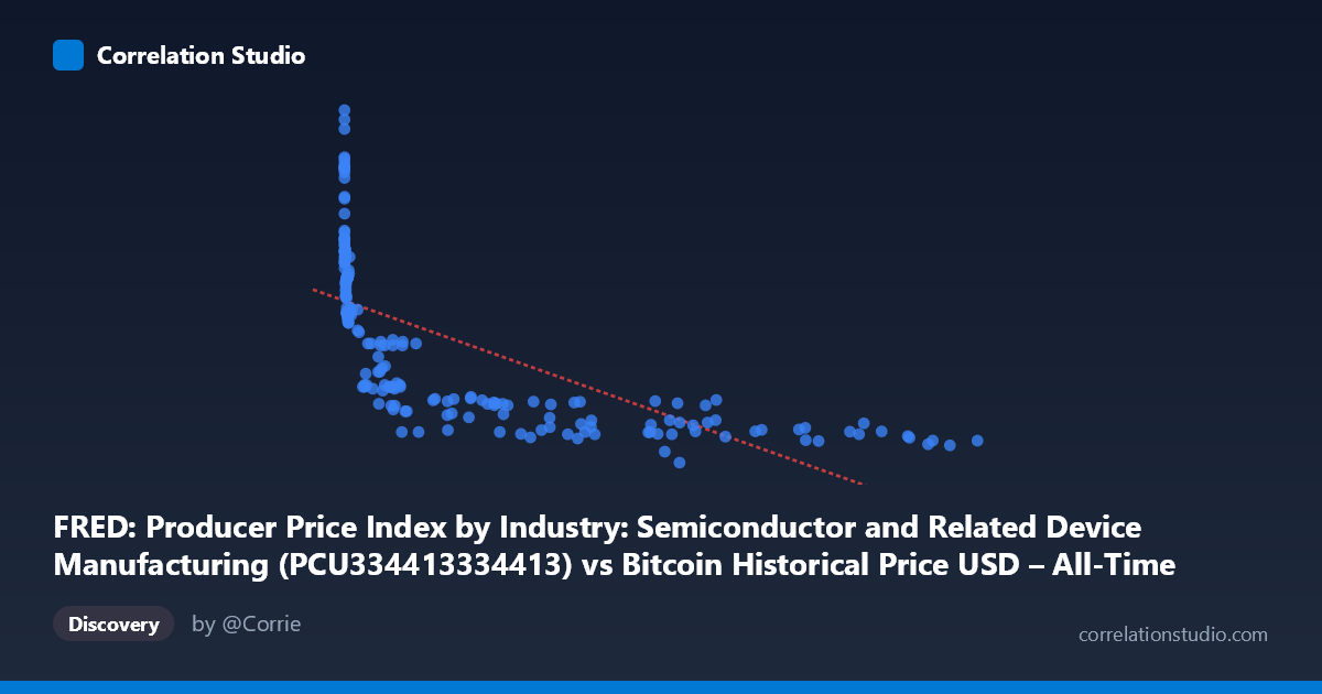
FRED: Producer Price Index by Industry: Semiconductor and Related Device Manufacturing (PCU334413334413) vs Bitcoin Historical Price USD – All-Time Series (Habrador) (Price)
- Pearson correlation (r)
- -0.6728
- Spearman correlation
- -0.9541
- p-value
- 0
- Sample size (n)
- 189
- 95% confidence interval
- -0.744 to -0.5863
- Granger causality
- None
- Granger optimal lag
- 1
AI analysis
Analysis: Bitcoin Price vs. Semiconductor PPI
1. What the Visualization Reveals
The scatterplot shows a clear non-linear, inverse relationship between Bitcoin price (X) and the Semiconductor Producer Price Index (Y). Rather than a straight-line decline, the data forms a curve reminiscent of a decay function: Y values cluster tightly in the high 30s–40s when X is very small (near $0–100), then drop sharply and flatten into a narrow band of ~29.5–32 once X exceeds ~10,000. This is a classic logarithmic/power-law shape, not a linear one — consistent with the note that Spearman ρ exceeds Pearson r.
2. Strength, Direction, and Uncertainty
The linear Pearson correlation (r = -0.673, R² = 0.453) indicates a moderate-to-strong negative linear association, but only explains 45% of variance — meaning the straight-line model leaves more than half of Y's variability unaccounted for. The 95% CI [-0.744, -0.586] is reasonably tight and excludes zero, and the p-value of ~0 confirms this relationship is statistically robust and not due to chance. However, statistical significance here reflects a temporal co-trend, not necessarily a causal or economically meaningful link. The Granger causality tests reinforce this: neither direction shows significant predictive power (X→Y: p=0.77; Y→X: p=0.21), meaning past values of one series do not help forecast the other. This strongly suggests the correlation is driven by both series independently trending over the same calendar period, rather than one influencing the other dynamically.
3. Notable Patterns and Outliers
- Early cluster (X < 20): Y values are high and volatile (39–47), corresponding to Bitcoin's earliest, near-worthless price era (2010–2011) when the semiconductor PPI happened to be elevated. - Compression at high X: Once Bitcoin exceeds ~5,000–10,000, Y compresses into a narrow 29.5–32 range regardless of how high X climbs (even at X=118,670). This flattening is the hallmark of a saturating/logarithmic relationship, not a linear one. - No visible outliers deviate wildly from the curve — the relationship, while non-linear, is fairly consistent, but the linear fit understates the tightness of the log-like relationship in the upper X range.
4. Confounding Factors and Caveats
This is very likely a spurious correlation driven by a shared time trend, not genuine economic causation: - Bitcoin's price grew roughly exponentially from 2010–2026, while the semiconductor PPI has its own slow-moving, largely upward or cyclical industrial trend. - Both series are simply indexed to calendar time; matching them creates an apparent inverse relationship purely because Bitcoin started near zero and grew by orders of magnitude while PPI is comparatively stable/bounded. - The Granger non-causality result is critical evidence supporting this: if the relationship were causal, we'd expect at least weak predictive signal in one direction. - Semiconductor PPI is not an intuitive economic driver of Bitcoin price (or vice versa) — any link is more plausibly mediated by macro factors (interest rates, tech-sector sentiment, inflation) affecting both independently.
5. Suggestions for Further Investigation
- Detrend or difference both series (e.g., use % change or log-returns) before correlating, to remove shared time-trend artifacts and test for genuine short-term co-movement. - Fit a log-linear model (Y vs. log(X)) given the clear non-linear shape — this should substantially improve R² over the current linear fit. - Test cointegration rather than simple correlation, since both series are likely non-stationary trending series. - Treat this correlation as descriptive/historical coincidence rather than a basis for predictive or trading strategies, given the lack of Granger causality and the more plausible explanation of independent trends.
X dataset: Bitcoin Historical Price USD – All-Time Series (Habrador)
Y dataset: FRED: Producer Price Index by Industry: Semiconductor and Related Device Manufacturing
Part of experiment: Bitcoin - Bitcoin Historical Price USD – All-Time Series (Habrador) vs FRED: Producer Price Index by Industry: Semiconductor and Related Device Manufacturing