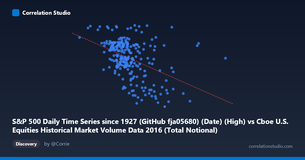
S&P 500 Daily Time Series since 1927 (GitHub fja05680) (Date) (High) vs Cboe U.S. Equities Historical Market Volume Data 2016 (Total Notional)
- Pearson correlation (r)
- -0.4429
- Spearman correlation
- -0.4401
- p-value
- 0
- Sample size (n)
- 252
- 95% confidence interval
- -0.5371 to -0.3378
- Granger causality
- None
- Granger optimal lag
- 1
AI analysis
Analysis: S&P 500 Daily High vs. Cboe Total Notional Volume (2016)
Relationship Overview The scatterplot reveals a moderate negative relationship between the S&P 500 daily high price and the total notional value of U.S. equity market volume traded on Cboe exchanges throughout 2016. As the S&P 500 daily high increases, total notional trading volume tends to decrease — a somewhat counterintuitive finding at first glance. The linear regression equation (y = -1.02×10⁻⁸x + 2297.63) confirms this inverse slope, suggesting that higher index price levels were associated with relatively quieter notional volume days during this period.
Correlation Strength and Statistical Significance The Pearson correlation of r = -0.4429 indicates a moderate negative association, but the explanatory power is modest: r² = 0.196, meaning only about 19.6% of the variance in total notional volume is explained by the S&P 500 daily high. The remaining ~80% is driven by other factors entirely. The 95% confidence interval of [-0.537, -0.338] is reasonably tight and does not cross zero, and the p-value of 1.57×10⁻¹³ confirms the correlation is highly statistically significant — virtually impossible to attribute to chance sampling. However, statistical significance here is partly a function of the relatively large sample (n = 252 full trading days), so practical significance should be interpreted cautiously given the limited variance explained. Notably, Granger causality tests found no significant directional predictive relationship in either direction (X→Y: F = 0.70, p = 0.40; Y→X: F = 0.22, p = 0.64), meaning that knowing today's S&P 500 high does not meaningfully improve prediction of tomorrow's notional volume, and vice versa. This suggests the correlation is contemporaneous and associative, not temporally predictive.
Notable Patterns and Outliers Several features stand out in the data. There is a visible clustering of points in the X range of roughly 16–21 billion, where notional volume spans broadly from ~2050 to ~2220, suggesting high variability in trading activity even when index levels are similar. At higher index values (above ~23–25 billion), notional volume tends to compress toward lower values (1850–1950 range), which drives much of the negative correlation signal. A handful of apparent outliers are worth noting: the point near (13.9B, 2271) shows very high notional volume at a relatively low index level, and points near (25B, 1890) and (40.9B — the extreme X outlier implied by the range) anchor the lower-right portion of the distribution. The extreme maximum X value of ~40.98B is far beyond the bulk of the distribution and likely represents a volatility spike day that could exert disproportionate leverage on the regression fit.
Confounding Factors and Caveats Several important caveats apply. First, 2016 was not a typical market year — it included significant macro events (Brexit in June, U.S. presidential election in November) that simultaneously affected both price levels and trading volumes in ways that may not generalize. Second, the axis labels appear swapped in the dataset metadata (X is labeled as S&P 500 "Date/High" from a volume dataset, and Y as "Total Notional" from the S&P dataset), suggesting a possible dataset join or labeling inconsistency that warrants verification before drawing firm conclusions. Third, notional volume is itself a function of price (shares × price), so using the S&P 500 price level as a predictor of notional volume introduces a mechanical or tautological element — higher prices naturally inflate notional values, making the observed negative relationship more surprising and potentially reflecting a compositional artifact. Finally, omitted variables such as VIX (volatility index), macroeconomic announcements, and sector rotation are likely significant drivers of both variables.
Actionable Insights and Further Investigation Given the modest explanatory power and absence of Granger causality, this correlation should not be used as a standalone predictive signal. However, several follow-up analyses are warranted: (1) Incorporate VIX or realized volatility as a covariate — it likely mediates the relationship, with low-volatility/high-price regimes suppressing trading activity; (2) Segment the data by market regime (pre/post-Brexit, pre/post-election) to test whether the negative relationship is driven by specific episodes; (3) Resolve the dataset labeling ambiguity to ensure the correct columns are being paired; (4) Test non-linear models, as the scatterplot hints at a possible threshold effect where the negative relationship strengthens above certain index levels; and (5) Examine share volume separately from notional volume to disentangle the price-level mechanical effect from genuine changes in trading activity.
X dataset: Cboe U.S. Equities Historical Market Volume Data 2016
Y dataset: S&P 500 Daily Time Series since 1927 (GitHub fja05680) (Date)
Part of experiment: Daily - Cboe U.S. Equities Historical Market Volume Data 2016 vs S&P 500 Daily Time Series since 1927 (GitHub fja05680) (Date)