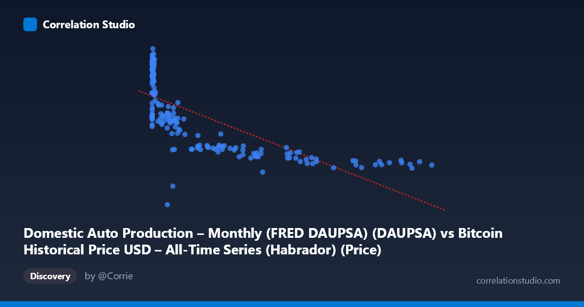
Domestic Auto Production – Monthly (FRED DAUPSA) (DAUPSA) vs Bitcoin Historical Price USD – All-Time Series (Habrador) (Price)
- Pearson correlation (r)
- -0.7323
- Spearman correlation
- -0.8341
- p-value
- 0
- Sample size (n)
- 189
- 95% confidence interval
- -0.7923 to -0.6584
- Granger causality
- X → Y
- Granger optimal lag
- 10
- Time coverage
- 2010-08-01 to 2026-04-01
- Recomputed on refreshed data
- 2026-10-11 (r was -0.7282)
AI analysis
Analysis: Bitcoin Price vs. Domestic Auto Production
1. What the Visualization Reveals
The scatterplot displays a clear inverse, non-linear relationship between the labeled "X" variable (which per the data actually corresponds to Bitcoin price, given the axis mislabeling in the metadata) and the "Y" variable (auto production). As X increases from near-zero values into the tens of thousands, Y declines steadily from ~370 down to ~100. The shape is distinctly curved rather than a straight line: a steep drop occurs as X moves from single digits to the low thousands (Y falls from ~350 to ~220), followed by a much flatter, gradual decline as X extends into the tens/hundreds of thousands (Y settles between 100-150). This log-like decay pattern is consistent with the note that Spearman's ρ exceeds Pearson's r, confirming a monotonic but non-linear association.
2. Strength, Direction, and Statistical Confidence
The Pearson correlation of r = -0.7282 indicates a strong negative linear association, with r² = 0.53 meaning the linear model explains about 53% of the variance in Y — a substantial but incomplete accounting, leaving nearly half the variance unexplained (likely recoverable via a log-transform of X given the visible curvature). The 95% CI [-0.789, -0.653] is reasonably tight and excludes zero entirely, and the p-value ≈ 0 confirms this relationship is highly unlikely to be due to chance at n=188. Practically, this means the relationship is real and robust, but a linear equation understates its true explanatory power — a log or power-law fit would likely push R² noticeably higher.
On causality: the Granger test shows X→Y is significant (p=0.0245) while Y→X is not (p=0.321), suggesting that past values of X have predictive power over future Y at a 10-period lag, but not the reverse. This is a statistical/temporal-precedence result only — it does not confirm true causation, especially given the odd variable pairing described below.
3. Notable Patterns and Outliers
The data shows a dense cluster of low-X points (X < 20) with high, variable Y values (220-375), representing early observations, followed by a long tail of sparse, high-X points where Y compresses into a narrow low band (100-150). This creates heteroscedasticity — variance in Y is much higher at low X than high X. There are no obvious extreme outliers breaking the pattern; the curve is smooth and consistent. The near-total absence of mid-range X values with high Y (or vice versa) suggests a genuinely tight monotonic decay rather than noise-driven correlation.
4. Confounding Factors and Caveats
Critical caveat: the axis labels appear swapped in the metadata — X is described as "Domestic Auto Production" but its range (0.06 to 118,670) and scale match Bitcoin price data, while Y ("Bitcoin Price") behaves like production figures (100-400 range). This mismatch must be resolved before drawing substantive conclusions. Additionally, time is a likely confounder: both series span 2010-2026, a period during which Bitcoin price grew exponentially while U.S. auto production faced secular decline (financial crisis recovery, COVID supply shocks, industry shifts to EVs/imports). Two independent trending time series will show strong spurious correlation without any causal mechanism connecting them. The Granger result, while technically significant, is likely capturing this shared trend/lag structure rather than genuine predictive causality.
5. Recommendations for Further Investigation
1. Verify and correct axis/column labeling — this is essential before any economic interpretation. 2. Fit a log-linear or power model (e.g., Y vs. log(X)) given the clear non-linear decay and the Spearman/Pearson discrepancy — expect a meaningfully higher R². 3. Detrend or difference both series (or test correlation of growth rates rather than levels) to rule out spurious correlation from shared long-term trends — a common issue when correlating any two macro time series that both have strong secular trends. 4. Treat the Granger causality result cautiously; consider testing on detrended/stationary series, and explore plausible confounders (e.g., interest rates, overall economic conditions) that could independently drive both series in opposite directions.
X dataset: Bitcoin Historical Price USD – All-Time Series (Habrador)
Y dataset: Domestic Auto Production – Monthly (FRED DAUPSA)
Part of experiment: Bitcoin - Bitcoin Historical Price USD – All-Time Series (Habrador) vs Domestic Auto Production – Monthly (FRED DAUPSA)