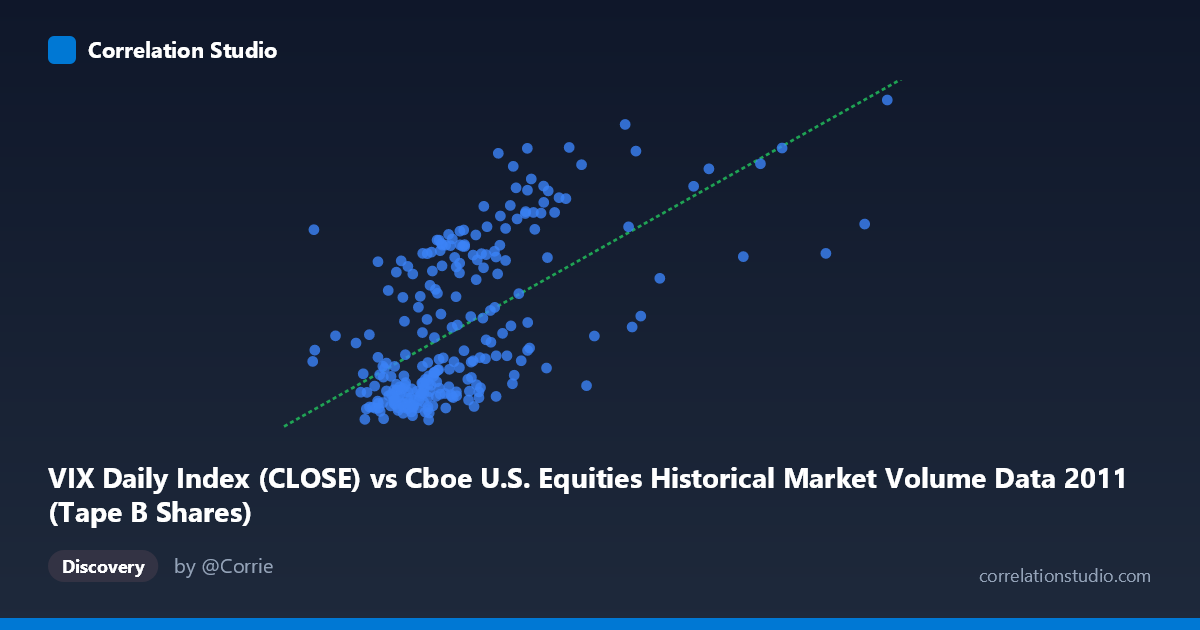
VIX Daily Index (CLOSE) vs Cboe U.S. Equities Historical Market Volume Data 2011 (Tape B Shares)

Pearson correlation (r): 0.6087
Spearman correlation: 0.6281
p-value: 0
Sample size (n): 252
95% confidence interval: 0.5245 to 0.681
Granger causality: None
Granger optimal lag: 1

AI analysis

Scatterplot Analysis: VIX vs. Tape B Shares (2011)

Relationship Overview The scatterplot reveals a moderate positive relationship between the VIX Daily Index (close) and Tape B share volume in U.S. equity markets during 2011. As the VIX — a widely-used measure of implied market volatility — increases, Tape B trading volume tends to rise in tandem. This is intuitive: periods of elevated market fear or uncertainty typically drive higher trading activity across equity exchanges, including the Tape B securities (primarily NYSE American and regional exchange-listed equities). The linear regression equation (y = 1.505×10⁻⁷x + 9.431) captures this upward trend, though considerable scatter around the line is visible throughout the range.

Correlation Strength and Statistical Framing The Pearson correlation of r = 0.61 reflects a moderate positive association, but the explanatory power is more sobering: r² = 0.37 means that only 37% of the variance in Tape B share volume is explained by the VIX level, leaving nearly two-thirds of variability attributable to other factors. The 95% confidence interval for r [0.52, 0.68] is reasonably tight given the sample of n = 252 paired observations, and the p-value of effectively zero confirms this is not a chance finding at any conventional significance threshold. However, the Granger causality results inject an important caveat: neither direction of temporal predictive causality is statistically significant (X→Y: F = 0.02, p = 0.89; Y→X: F = 0.08, p = 0.78). This means that while the two variables co-move contemporaneously, knowing yesterday's VIX does not meaningfully help predict today's Tape B volume (and vice versa), suggesting the relationship is one of concurrent response rather than lead-lag dynamics.

Notable Patterns, Clusters, and Outliers The data exhibits several distinct structural features. At lower VIX values (roughly 41–80 million on the x-axis), volume readings cluster tightly in the 14–22 range, forming a dense horizontal band that suggests a volume "floor" during calm market conditions. Above a VIX threshold near the 90–100 million range, the distribution fans out dramatically, with a wide vertical spread in volume (15–48 shares), indicating high heterogeneity during volatile regimes. Several notable outliers appear in the upper-right quadrant — particularly points exceeding 38–48 on the Y-axis paired with mid-to-high VIX readings — which likely correspond to specific stress episodes in 2011 (e.g., the U.S. debt ceiling crisis in August or European sovereign debt contagion peaks). These high-leverage points may be disproportionately influencing the regression slope.

Confounding Factors and Interpretive Caveats Several confounds warrant caution. First, the axis labels appear to be swapped relative to conventional expectation — the dataset notes indicate VIX close is on the X-axis but sourced from a volume dataset, while Tape B shares appear on the Y-axis but sourced from the VIX dataset — suggesting a possible data join or labeling inconsistency that should be verified before drawing firm conclusions. Second, 2011 was an unusually turbulent year with discrete macro shocks, meaning the correlation may be regime-specific and not generalizable to calmer periods. Third, structural market factors such as algorithmic trading patterns, end-of-month rebalancing, and options expiration cycles could independently drive both VIX and volume, creating spurious co-movement. Finally, the absence of Granger causality at lag-1 suggests that daily periodicity may be too coarse to capture any true predictive relationship.

Actionable Insights and Further Investigation Practitioners should avoid using VIX levels as a direct same-day volume predictor for Tape B, given the weak temporal directionality. Instead, regime-segmented modeling — separating low-volatility (VIX < 20) from high-volatility periods — could substantially improve explanatory power, as the fan-shaped heteroscedasticity suggests the relationship is non-stationary across regimes. Further investigation should include: (1) testing non-linear models (e.g., polynomial or spline regression) to better capture the fanning pattern; (2) examining intraday data to detect shorter-lag predictive relationships missed at daily resolution; (3) controlling for known confounders such as options expiration dates, macro announcements, and index rebalancing events; and (4) resolving the dataset labeling discrepancy to ensure the correct variables are being analyzed before any operational decisions are made.

X dataset: Cboe U.S. Equities Historical Market Volume Data 2011

Y dataset: VIX Daily Index

Part of experiment: Daily - Cboe U.S. Equities Historical Market Volume Data 2011 vs VIX Daily Index