IMF Primary Commodity Prices – Monthly Time Series (53 Commodities, 10 Indexes) (Soybean Oil) vs Bitcoin Historical Price USD – All-Time Series (Habrador) (Price)
- Pearson correlation (r)
- -0.5994
- Spearman correlation
- -0.7138
- p-value
- 0
- Sample size (n)
- 83
- 95% confidence interval
- -0.7218 to -0.4406
- Granger causality
- None
- Granger optimal lag
- 10
- Time coverage
- 2010-08-01 to 2017-06-01
- Recomputed on refreshed data
- 2026-10-24 (r was -0.5994)
AI analysis
Analysis: Soybean Oil Price Index vs. Bitcoin Historical Price
1. Overview of the Relationship
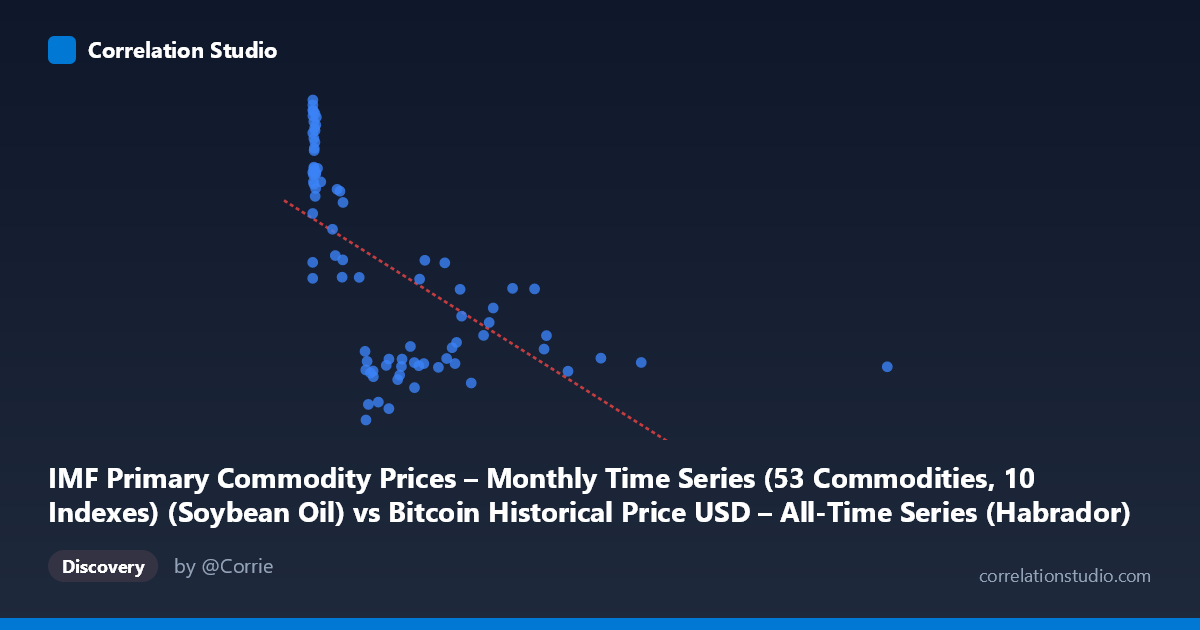
The scatterplot displays a moderate negative association between soybean oil commodity prices (X-axis) and Bitcoin price (Y-axis) across 83 paired monthly observations spanning 2010–2017. The data cloud shows a clear downward-sloping tendency, but with substantial vertical scatter at low X-values, where the majority of points are concentrated (X range 0–500, given mean of 321 and heavy right-skew toward the max of 2452). This clustering at low X with wide Y-dispersion (roughly 590–1279) suggests the relationship is not uniform across the full range of soybean oil prices.
2. Strength, Direction, and Statistical Confidence
The Pearson correlation coefficient of r = -0.599 indicates a moderate negative linear relationship: as soybean oil prices rise, Bitcoin prices tend to fall (or vice versa, given no causal direction is established). However, r² = 0.359 means only about 36% of the variance in Bitcoin price is explained by soybean oil price in this linear model — the majority of Bitcoin's price variation (64%) is driven by other factors entirely. The 95% confidence interval [-0.722, -0.441] is reasonably tight and does not cross zero, and the p-value (2.14×10⁻⁹) is highly significant, giving strong confidence that a real negative association exists in this sample — but statistical significance here reflects strength of evidence for correlation, not causation or practical predictive power. Critically, the Granger causality tests show no significant predictive direction in either direction (X→Y: p=0.375; Y→X: p=0.079, only marginally suggestive). This strongly indicates the correlation is not driven by one variable temporally leading the other — it's more likely a spurious or confound-driven relationship, possibly both series independently trending over the 2010–2017 window.
3. Notable Patterns and Outliers
Several features stand out: (a) a dense cluster of points near X≈0–20 with Y values spanning nearly the entire range (590–1279), representing many early low-soybean-oil-price months coinciding with highly variable Bitcoin prices during Bitcoin's early volatile history; (b) a sparse tail of high-X outliers (e.g., X=1402, X=2452) that sit at moderate-low Y values (~700), which have disproportionate leverage on the linear fit; (c) the note that Spearman's ρ exceeds Pearson's r suggests a monotonic but non-linear (possibly logarithmic or power-law) relationship fits better — plausible given Bitcoin's known exponential growth phases and the compressed, skewed distribution of the commodity index.
4. Confounding Factors and Caveats
This is very likely a spurious correlation driven by shared time trends rather than any economic mechanism linking soybean oil and Bitcoin. Both series were sampled over the same 2010–2017 period, during which Bitcoin underwent extreme secular price growth and commodity indexes fluctuated due to unrelated macro factors (global demand, weather, biofuel policy). Time-series data like this often exhibit "nonsense regression" due to autocorrelation and non-stationarity — neither series is likely stationary, which inflates correlation estimates. The lack of Granger causality reinforces that this is probably coincidental co-trending, not a functional relationship. Additionally, small sample size (n=83 monthly points vs. population of 449) and uneven X-distribution (heavily right-skewed with extreme outliers) can distort both r and the regression slope.
5. Recommendations for Further Investigation
To determine whether this relationship is meaningful or spurious: (1) test both series for stationarity (ADF/KPSS tests) and consider differencing or detrending before correlating; (2) re-run correlation on log-transformed or detrended series to remove shared trend artifacts; (3) explore the suggested non-linear fits (log-log or polynomial) given the Spearman/Pearson divergence; (4) control for known Bitcoin-specific drivers (halving cycles, exchange volume, regulatory news) and commodity-specific drivers (biofuel mandates, crop yields) to check if the relationship survives after removing common macro trends (e.g., USD strength, global risk sentiment); (5) given the non-significant Granger results, avoid using soybean oil prices as a predictive feature for Bitcoin price forecasting models without further validation.
X dataset: Bitcoin Historical Price USD – All-Time Series (Habrador)
Y dataset: IMF Primary Commodity Prices – Monthly Time Series (53 Commodities, 10 Indexes)
Part of experiment: Bitcoin - Bitcoin Historical Price USD – All-Time Series (Habrador) vs IMF Primary Commodity Prices – Monthly Time Series (53 Commodities, 10 Indexes)