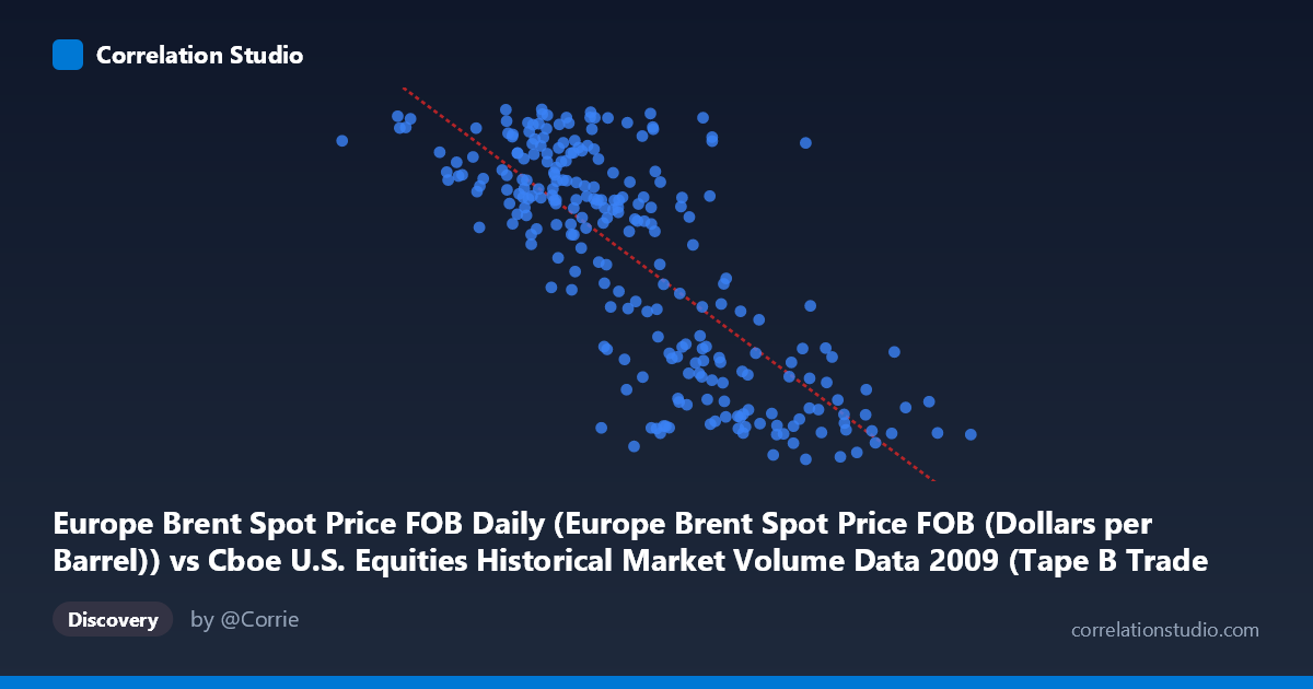
Europe Brent Spot Price FOB Daily (Europe Brent Spot Price FOB (Dollars per Barrel)) vs Cboe U.S. Equities Historical Market Volume Data 2009 (Tape B Trade Count)
- Pearson correlation (r)
- -0.7718
- Spearman correlation
- -0.7447
- p-value
- 0
- Sample size (n)
- 252
- 95% confidence interval
- -0.8175 to -0.7166
- Granger causality
- None
- Granger optimal lag
- 1
- Time coverage
- 2009-01-02 to 2009-12-31
- Recomputed on refreshed data
- 2026-11-12 (r was -0.7718)
AI analysis
Analysis: Europe Brent Spot Price vs. Cboe Tape B Trade Count (2009)
Relationship Overview The scatterplot reveals a clear negative relationship between Europe Brent Spot Price (FOB, USD/barrel) and Cboe Tape B Trade Count across 2009 trading days. As oil prices rise, U.S. equity trade counts on Tape B (primarily NYSE American and regional exchanges) tend to fall, and vice versa. The linear regression equation (y = -7.64×10⁻⁵x + 92.43) quantifies this inverse slope, with the fitted line cutting meaningfully across the data cloud from upper-left to lower-right. The data span a substantial range — oil prices from ~$82 to ~$767 per notional unit and trade counts from ~39 to ~79 — giving the relationship considerable dynamic range to express itself visually.
Correlation Strength and Statistical Significance The Pearson correlation of r = -0.7718 indicates a strong negative association, and the R² of 0.5957 means that approximately 59.6% of the day-to-day variance in Tape B trade counts is statistically explained by oil price levels — a notably high figure for two seemingly disparate financial series. The 95% confidence interval of [-0.8175, -0.7166] is tight and sits entirely in negative territory, reflecting high statistical confidence in the direction and approximate magnitude of this relationship. The p-value of ~0 (against an N of 3,232) confirms this is not a chance artifact. However, the Granger causality tests tell a more cautionary story: neither direction (X→Y: F=0.0096, p=0.922; Y→X: F=1.956, p=0.163) reaches statistical significance at any conventional threshold. This means that while the two series are strongly contemporaneously correlated, neither one reliably predicts the other one period ahead — the relationship is associative and likely driven by common underlying forces rather than one series mechanistically causing the other.
Patterns, Clusters, and Outliers The scatterplot shows a moderately tight but heteroscedastic cloud: at lower X values (oil prices roughly 80–300), trade counts are broadly elevated (55–78 range) with considerable vertical scatter, while at higher X values (500–770), trade counts compress toward the 40–55 range with less dispersion. This funnel-like spread suggests the negative relationship may be somewhat non-linear — possibly logarithmic or hyperbolic — with diminishing sensitivity at extreme oil prices. A few notable outliers are visible: points like (766,763, 42.19) and (662,859, 41.27) sit at extreme high-X/low-Y positions consistent with the trend, while (284,114, 77.18) and (474,940, 77.74) show high trade counts at mid-range oil prices. No dramatic outliers break the overall pattern, but the cluster of high-activity days all occurring at lower oil price levels is structurally notable.
Confounding Factors and Caveats The most significant interpretive caveat is that 2009 was a highly unusual year — it encompassed the tail of the Global Financial Crisis, a market bottom in March, and a strong recovery rally, all accompanied by dramatic swings in risk appetite, volatility (VIX), and trading volumes. Oil prices in 2009 recovered from crisis lows to mid-cycle levels, while equity market structure was simultaneously shifting with high-frequency trading growth. Both variables likely share a common driver in macro risk sentiment: when fear and uncertainty were highest (early 2009, low oil prices), equity trading volumes surged as investors repositioned; as confidence returned (higher oil prices), volumes normalized. This classic "risk-on/risk-off" dynamic, rather than any direct oil-equity mechanism, likely underpins the correlation. Additionally, Tape B trade count specifically captures smaller/regional exchange activity, which may respond differently to macro conditions than consolidated market volume.
Actionable Insights and Further Investigation Given the absence of Granger causality, practitioners should not use oil prices as a leading indicator for Tape B trade counts (or vice versa) in a short-term trading or operations context. However, the strong contemporaneous correlation warrants investigating a latent common factor — likely a volatility index (VIX), credit spreads, or a macro sentiment composite — that drives both series simultaneously. Further analysis should: (1) introduce VIX or economic uncertainty indices as control variables to test whether the oil–volume correlation survives partial correlation analysis; (2) test for non-linear functional forms (log-log or piecewise regression) given the apparent heteroscedasticity; (3) extend the time series beyond 2009 to determine whether this relationship is structurally persistent or a crisis-era artifact; and (4) decompose Tape B volume by market phase (pre-crisis, crisis, recovery) to identify whether the correlation is regime-dependent. The finding is statistically robust but economically requires a richer causal framework before any operational or investment conclusions can be drawn.
X dataset: Cboe U.S. Equities Historical Market Volume Data 2009
Y dataset: Europe Brent Spot Price FOB Daily
Part of experiment: Daily - Cboe U.S. Equities Historical Market Volume Data 2009 vs Europe Brent Spot Price FOB Daily