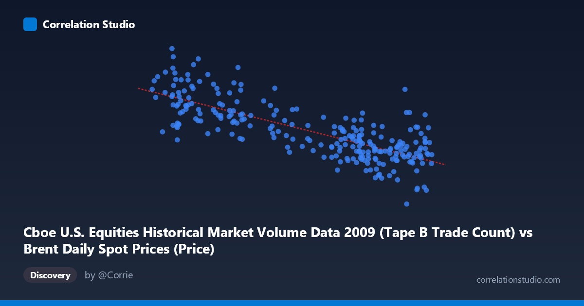
Cboe U.S. Equities Historical Market Volume Data 2009 (Tape B Trade Count) vs Brent Daily Spot Prices (Price)
- Pearson correlation (r)
- -0.7718
- Spearman correlation
- -0.7447
- p-value
- 0
- Sample size (n)
- 252
- 95% confidence interval
- -0.8175 to -0.7166
- Granger causality
- None
- Granger optimal lag
- 10
AI analysis
Scatterplot Analysis: Cboe Tape B Trade Count vs. Brent Crude Oil Spot Price (2009)
Relationship Overview
The scatterplot reveals a moderately strong negative relationship between Cboe U.S. Equities Tape B trade count and Brent crude oil spot prices across 2009. As equity trade volume increases, Brent crude prices tend to decline, and vice versa. The linear regression equation (y = -7,800.57x + 883,439) quantifies this inverse slope: each additional unit of trade count is associated with roughly a $7,800 decrease in the Brent spot price. Visually, the data cloud tilts clearly from upper-left to lower-right, confirming the negative trend, though with considerable scatter around the regression line indicating the relationship is real but imperfect.
Correlation Strength and Statistical Framing
The Pearson correlation of r = -0.7718 indicates a strong negative association, and the r² of 0.5957 means that approximately 59.6% of the variance in Brent crude prices is statistically explained by Tape B trade count — a substantial but not dominant share, leaving ~40% attributable to other factors. The 95% confidence interval of [-0.8175, -0.7166] is relatively narrow and does not cross zero, reflecting high precision in this estimate given the large sample (n = 252 paired observations from a population of 3,232). The p-value of effectively 0 confirms this correlation is overwhelmingly unlikely to be a chance artifact. However, the Granger causality tests find no significant predictive direction in either direction (X→Y: F = 1.85, p = 0.053; Y→X: F = 1.43, p = 0.168), meaning that neither variable reliably predicts the other's future values temporally, even at an optimal lag of 10 periods. This is a critical caveat: the correlation is robust cross-sectionally, but it does not imply a forecastable lead-lag relationship.
Notable Patterns, Clusters, and Outliers
Several features stand out in the data: - Outliers on the extremes: The point at approximately (42.19, 766,763) represents an exceptionally high Brent price paired with very low trade volume, sitting well above the regression line. Similarly, (75.15, 81,703) — the lowest Brent price in the dataset — falls far below the trend at high volume, both likely corresponding to unusual market days in early 2009. - Clustering at low trade counts (40–50 range): Y-values here span an enormous range (~418K to ~767K), suggesting high price volatility during low-volume periods, possibly reflecting the volatile early-2009 oil market recovery from the 2008 financial crisis lows. - Compression at high trade counts (70–78 range): Brent prices cluster more tightly between ~150K–490K, indicating relatively more predictable pricing during high-volume periods. - There is a hint of heteroscedasticity — variance in Y appears larger at lower X values — which slightly undermines the assumptions of ordinary linear regression.
Confounding Factors and Caveats
This correlation almost certainly reflects shared temporal dynamics rather than a direct causal mechanism between equity trade volume and crude oil prices. Both variables evolved dramatically throughout 2009: Brent crude recovered from ~$40/barrel in January to ~$78/barrel by December, while equity market volumes followed their own structural trajectory post-financial crisis. This creates a spurious time-trend confound — two variables moving in opposite directions over the same year will appear correlated even without any direct link. Additionally, the dataset pairing is conceptually unusual; Tape B specifically covers regional U.S. equity exchanges, which have no obvious direct fundamental connection to European crude oil pricing. Seasonal effects, macroeconomic sentiment, and USD exchange rate fluctuations could all be driving both series simultaneously.
Actionable Insights and Further Investigation
Despite the absence of Granger causality, the strong cross-sectional correlation warrants deeper investigation: 1. Detrend both series by removing the shared 2009 time trend (e.g., via first-differencing or residualization against date) to test whether the correlation persists beyond the common temporal trajectory. 2. Introduce macroeconomic controls — particularly the VIX (fear index), USD index, and S&P 500 returns — to identify whether a third variable drives both equity volume and oil prices simultaneously. 3. Examine the outliers (early January and specific shock days) to determine if they correspond to identifiable market events (e.g., OPEC announcements, earnings seasons) that could explain the extreme values. 4. Extend the analysis across multiple years to test whether this negative relationship is stable or unique to the 2009 post-crisis recovery environment. 5. Consider non-linear modeling (e.g., polynomial or piecewise regression) given the heteroscedasticity and potential regime differences between low- and high-volume trading environments.
X dataset: Brent Daily Spot Prices
Y dataset: Cboe U.S. Equities Historical Market Volume Data 2009
Part of experiment: Daily - Brent Daily Spot Prices vs Cboe U.S. Equities Historical Market Volume Data 2009