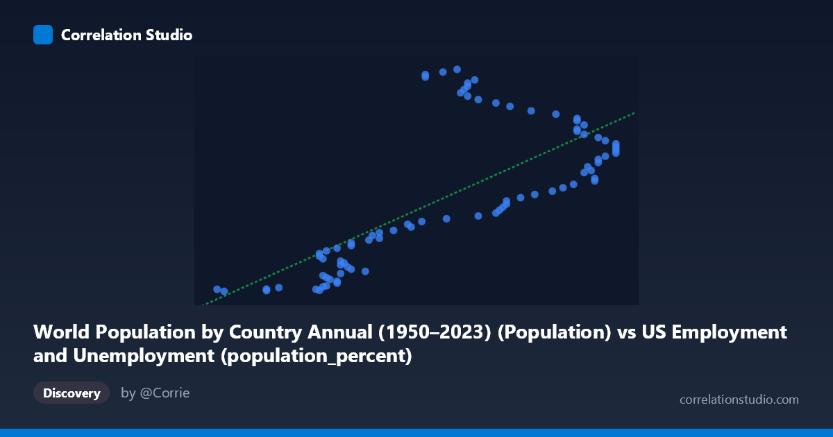
World Population by Country Annual (1950–2023) (Population) vs US Employment and Unemployment (population_percent)
- Pearson correlation (r)
- 0.7227
- Spearman correlation
- 0.7445
- p-value
- 0
- Sample size (n)
- 83
- 95% confidence interval
- 0.6006 to 0.8118
- Granger causality
- None
- Granger optimal lag
- 10
- Time coverage
- 1941-01-01 to 2023-01-01
AI analysis
Scatterplot Analysis: World Population vs. US Employment Population Percent
1. Overall Relationship The scatterplot reveals a positive, moderately strong relationship between the total world population (X-axis, drawn from US Employment/BLS data) and the US employment population percent expressed in absolute population terms (Y-axis). As world population increases across the 1941–2023 timeframe, the US employment-linked population metric rises correspondingly. The linear regression equation y = 8.29×10⁶x − 4.20×10⁸ suggests that for each unit increase in the population variable, the Y metric increases by approximately 8.3 million, though the substantial intercept offset highlights that the relationship only becomes meaningful across a narrow, high-value range of X (roughly 55.8 to 67.1, likely representing population in tens or hundreds of millions).
2. Correlation Strength and Statistical Significance The Pearson correlation of r = 0.7227 indicates a moderately strong positive association, but the R² of 0.5223 is the more sobering figure — it means that only ~52% of the variance in Y is explained by X, leaving nearly half the variation unaccounted for by this linear relationship alone. The 95% confidence interval for r [0.6006, 0.8118] is reasonably tight and does not approach zero, and the p-value of 1.22×10⁻¹⁴ confirms the correlation is highly statistically significant — essentially ruling out chance as an explanation. However, statistical significance should not be conflated with causal or practical meaningfulness, especially given the time-series nature of the data. Critically, the Granger causality analysis finds no significant predictive direction in either direction (X→Y: F=1.15, p=0.348; Y→X: F=1.64, p=0.122), meaning that past values of world population do not significantly help forecast the US employment metric beyond its own history, and vice versa. This strongly suggests the observed correlation is likely driven by a shared underlying trend (secular growth over time) rather than any direct causal mechanism.
3. Notable Patterns, Clusters, and Outliers Several features stand out in the data distribution. There appears to be a notable cluster of high-Y outliers at moderate X values — for example, points like (62.20, 161,811,336), (62.60, 163,211,907), (62.70, 150,873,433), and (63.10, 157,652,893) sit dramatically above the regression line, suggesting that certain years with mid-range population figures produced unusually high Y values. Conversely, many points in the X range of 58–61 cluster tightly near lower Y values with relatively low dispersion, while the upper X range (65–67) shows higher Y values but also increased scatter, indicating growing heteroscedasticity. This fanning pattern suggests the linear model's fit degrades at higher population values, and a non-linear (e.g., polynomial or exponential) model might better capture the underlying dynamics.
4. Confounding Factors and Caveats The most significant interpretive caveat is that both variables are time-indexed from 1941–2023, meaning much of the observed correlation almost certainly reflects parallel long-run temporal trends (world population grows over decades; US labor force metrics also trend upward) rather than any direct demographic-to-employment relationship. This is a textbook case of spurious correlation via shared temporal trend, and the Granger causality null result reinforces this interpretation. Additionally, the X-axis variable is labeled as coming from a US Employment dataset but represents world population — an unusual pairing that raises questions about data provenance and whether the column alignment across datasets is meaningful. The high-Y outlier cluster around X=62–63 may correspond to specific historical periods (possibly post-WWII boom years or specific BLS methodology changes) that introduce structural breaks. Finally, with n=83 of a possible N=86, a small number of missing observations could introduce selection bias if the gaps are non-random.
5. Actionable Insights and Further Investigation Given the unresolved variance (~48%) and the absence of Granger causality, several investigative steps are warranted. First, detrending both series (e.g., using first differences or a Hodrick-Prescott filter) before computing correlations would isolate cyclical co-movement from shared secular trends, providing a more honest measure of association. Second, the high-Y outlier cluster deserves specific attention — identifying which years these correspond to and whether they align with known labor market disruptions (e.g., WWII mobilization, Baby Boom, COVID-19) could reveal structural regime differences. Third, testing non-linear regression models (quadratic, logarithmic, or piecewise) is advisable given the visible heteroscedasticity and the outlier cluster. Fourth, introducing mediating variables — such as US GDP, labor force participation rate, or demographic age-structure data — could help decompose how much of the Y variance is attributable to domestic vs. global demographic forces. Ultimately, the correlation appears to be a time-trend artifact rather than a substantively causal relationship, and any policy or forecasting application should proceed with considerable caution.
X dataset: US Employment and Unemployment
Y dataset: World Population by Country Annual (1950–2023)
Part of experiment: Yearly - US Employment and Unemployment vs World Population by Country Annual (1950–2023)