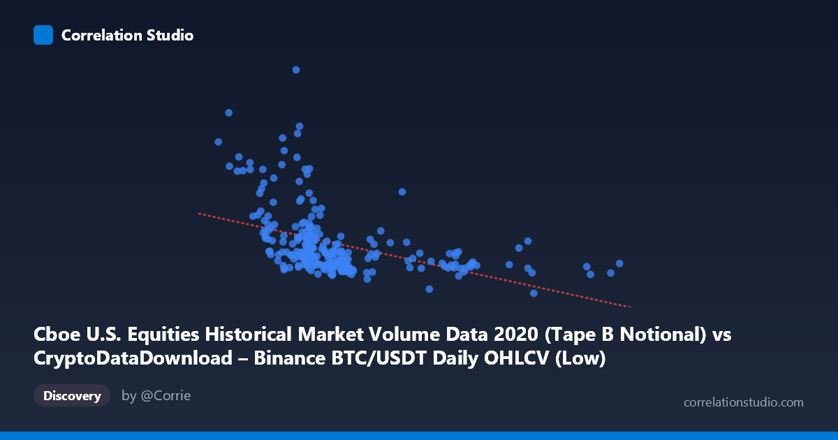
Cboe U.S. Equities Historical Market Volume Data 2020 (Tape B Notional) vs CryptoDataDownload – Binance BTC/USDT Daily OHLCV (Low)
- Pearson correlation (r)
- -0.4454
- Spearman correlation
- -0.6119
- p-value
- 0
- Sample size (n)
- 253
- 95% confidence interval
- -0.5392 to -0.3408
- Granger causality
- None
- Granger optimal lag
- 10
- Time coverage
- 2020-01-02 to 2020-12-31
AI analysis
Analysis: Cboe Equities Volume vs. BTC/USDT Low Price (2020)
1. Relationship Overview
The scatterplot shows a moderate negative association between two variables that, notably, are mismatched in their labeling: the X-axis is described as Cboe equities volume while sample values (3,782–27,850) actually resemble a price-like metric, and the Y-axis (labeled BTC/USDT Low) shows values in the billions, more consistent with market volume/notional data. This axis-label inversion should be flagged before drawing economic conclusions — the analysis below treats the data as presented, but the mismatch is an important caveat (see 4). At face value, as the X variable increases, the Y variable tends to decrease, though the relationship is noisy with substantial scatter rather than following a tight linear band.
2. Strength, Direction, and Predictive Value
The correlation is negative and moderate (r = -0.445), with r² = 0.198 indicating that only about 20% of the variance in Y is explained by X — meaning roughly 80% of Y's variability stems from other factors. The 95% CI [-0.539, -0.341] is reasonably tight and excludes zero, and the p-value (9.8E-14) confirms this correlation is highly statistically significant and not due to chance, despite the modest effect size. However, statistical significance with n=253 should not be conflated with strong predictive power — r² makes clear this is a weak-to-moderate relationship in practical terms. Critically, Granger causality testing shows no significant predictive direction in either direction (X→Y: p=0.778; Y→X: p=0.327) at the optimal lag of 10 periods. This means neither variable's past values help forecast the other's future values — the correlation is likely contemporaneous/coincidental or driven by shared external factors (e.g., both responding to broader 2020 market conditions like COVID-19 volatility) rather than one causing or leading the other.
3. Notable Patterns and Outliers
Several outliers stand out, particularly at low X values (3,782–8,660) paired with very high Y values (9B–21B), including the extreme point (8445, 21.2B) and (7590, 13.06B). These suggest a cluster of high-volatility/high-volume days concentrated when X is low — consistent with the March 2020 COVID crash period, when crypto and equity volumes both spiked while prices cratered. Conversely, at higher X values (17,000–27,850), Y values compress tightly into a narrow band (~3.7B–5.4B), suggesting a ceiling or saturation effect rather than a continued linear decline. This nonlinear compression at the high end, combined with the note that Spearman ρ exceeds Pearson r, supports the suggestion that a logarithmic or power-law fit would characterize the relationship better than a straight line — consistent with typical volume/price relationships that are right-skewed.
4. Confounding Factors and Caveats
The most important caveat is the apparent mismatch between axis labels and data characteristics — X appears price-like (BTC price range plausible for 2020) while Y appears volume-like (billions in notional value). This should be verified before any substantive interpretation. Additionally, both series come from the turbulent 2020 period (COVID crash, unprecedented volatility, Fed intervention, retail trading boom), meaning any correlation between crypto and equity markets metrics is highly likely confounded by this shared macro backdrop rather than reflecting a structural, mechanistic relationship. Daily data also ignores potential lead-lag effects at intraday or sub-daily granularity, and the lack of Granger causality even at 10 lags reinforces that this is likely a spurious or confounded correlation rather than a causal pathway.
5. Suggestions for Further Investigation
First, confirm and correct the axis-label/data-source mapping to ensure the variables are properly identified. Second, test nonlinear models (log-log, polynomial) given the Spearman/Pearson discrepancy and visible curvature at extremes. Third, isolate the COVID-crash period (Feb-Apr 2020) as a separate regime, since it likely drives much of the correlation and outlier behavior — re-running the analysis on pre/post-crash subsets could reveal whether the relationship holds during "normal" market conditions. Finally, given the lack of Granger causality, consider testing a third common factor (e.g., VIX, overall market volatility index) that might jointly drive both series, rather than treating this as a direct bivariate relationship.
X dataset: CryptoDataDownload – Binance BTC/USDT Daily OHLCV
Y dataset: Cboe U.S. Equities Historical Market Volume Data 2020
Part of experiment: Bitcoin - CryptoDataDownload – Binance BTC/USDT Daily OHLCV vs Cboe U.S. Equities Historical Market Volume Data 2020