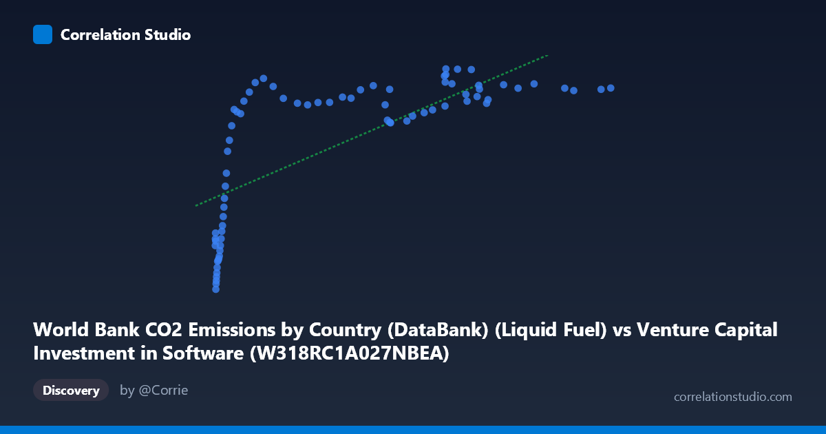
World Bank CO2 Emissions by Country (DataBank) (Liquid Fuel) vs Venture Capital Investment in Software (W318RC1A027NBEA)
- Pearson correlation (r)
- 0.719
- Spearman correlation
- 0.8188
- p-value
- 0
- Sample size (n)
- 75
- 95% confidence interval
- 0.5879 to 0.8132
- Granger causality
- None
- Granger optimal lag
- 10
- Time coverage
- 1946-01-01 to 2020-01-01
AI analysis
Scatterplot Analysis: Liquid Fuel CO2 Emissions vs. Venture Capital Investment in Software
1. Overall Relationship Pattern
The scatterplot reveals a moderately strong positive association between liquid fuel CO2 emissions and venture capital investment in software, but the relationship is strikingly non-linear. The data exhibits a clear logarithmic or saturation curve: at low X values (roughly 0–50 units), Y rises steeply and rapidly, while beyond approximately X = 100, Y plateaus into a relatively flat band clustered between ~11,000 and ~13,600. This suggests that the linear regression model (y = 18.32x + 7,113.14) is a reasonable first approximation but meaningfully misrepresents the true functional form of the relationship, likely overestimating Y at intermediate X values and underestimating it at low X values.
2. Correlation Strength, Explained Variance, and Granger Causality
The Pearson correlation of r = 0.719 indicates a moderate-to-strong positive correlation, but the r² of 0.517 is the more sobering statistic — it means that only about 51.7% of the variance in VC software investment is explained by liquid fuel emissions, leaving nearly half the variation unexplained by this single predictor. The 95% confidence interval of [0.588, 0.813] is reasonably tight and entirely positive, confirming directional confidence, and the p-value of 3.76×10⁻¹³ makes the association highly statistically significant — virtually ruling out chance as an explanation at any conventional threshold. However, the Granger causality results are unambiguous in their null finding: neither X→Y (F = 0.44, p = 0.918) nor Y→X (F = 0.81, p = 0.619) reaches significance at the optimal lag of 10 periods. This is a critical caveat — despite the strong contemporaneous correlation, neither variable temporally predicts the other, meaning the relationship is almost certainly driven by shared underlying trends (e.g., economic growth, industrialization) rather than any direct causal mechanism in either direction.
3. Notable Patterns, Clusters, and Outliers
The data segregates visually into two distinct behavioral regimes. The low-X cluster (X < ~50) spans a wide vertical range from roughly 2,500 to 13,000, producing most of the variance and driving the apparent correlation. Within this region, several notable low-end outliers — (1.53, 2497), (1.82, 2775), (2.11, 2937), (2.33, 3128) — anchor the lower-left of the plot and are consistent with early time periods or very low-emission economies. The high-X cluster (X ~100) forms a dense, nearly horizontal band around 11,000–13,600, showing very low variance in Y despite substantial variance in X, which is characteristic of a saturation effect. A handful of points near (0.85–1.33) show surprisingly high Y values (4,700–5,334), suggesting these may be early-period anomalies or data join artifacts that slightly distort the lower-bound trend.
4. Confounding Factors and Interpretive Caveats
The most significant caveat is that both variables are strongly time-trended: global CO2 emissions from liquid fuels have risen consistently since 1946, and VC investment in software has grown dramatically since the 1980s. A shared upward trend over 1946–2020 will mechanically produce positive correlation even when the two phenomena are causally unrelated — this is a classic spurious correlation driven by common secular trends. The dataset labeling also raises a concern: the X-axis is labeled as a column from "Venture Capital Investment in Software" but describes CO2 emissions data, and the Y-axis is the reverse — suggesting a possible dataset join or column assignment error that warrants verification before drawing any substantive conclusions. Additionally, the 10-period Granger lag structure (likely ~10 years) suggests limited short-term temporal linkage, further undermining a causal interpretation.
5. Actionable Insights and Further Investigation
Given the non-linear pattern, a log-linear or polynomial regression (e.g., fitting log(X) as a predictor) would almost certainly outperform the linear model and provide a more honest representation of the relationship. Before any further modeling, dataset column assignments should be audited to confirm that the correct variables are on each axis, as the metadata descriptions appear transposed. Analysts should consider detrending both series (e.g., via first differencing or HP filtering) prior to correlation analysis to remove the shared secular trend and test whether any residual association remains — if the correlation collapses after detrending, the relationship is likely spurious. If a genuine relationship is hypothesized (e.g., industrialization driving both emissions and tech investment), a multivariate framework controlling for GDP, population, and decade fixed effects would be the appropriate next step. Finally, the Granger null result should discourage any policy or forecasting application that assumes one variable can predict the other across time.
X dataset: Venture Capital Investment in Software
Y dataset: World Bank CO2 Emissions by Country (DataBank)
Part of experiment: Yearly - Venture Capital Investment in Software vs World Bank CO2 Emissions by Country (DataBank)