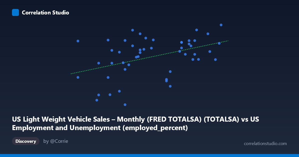
US Light Weight Vehicle Sales – Monthly (FRED TOTALSA) (TOTALSA) vs US Employment and Unemployment (employed_percent)
- Pearson correlation (r)
- 0.4228
- Spearman correlation
- 0.4
- p-value
- 0.002222
- Sample size (n)
- 50
- 95% confidence interval
- 0.1637 to 0.6273
- Granger causality
- None
- Granger optimal lag
- 1
AI analysis
Analysis of US Light Vehicle Sales vs. Employment Rate
Relationship Overview The scatterplot reveals a modest positive relationship between US Light Weight Vehicle Sales (X-axis, in millions of units SAAR) and the US Employment Percentage (Y-axis). As vehicle sales increase, employment rates tend to rise slightly, which is directionally intuitive given that auto sales are both a reflection of consumer confidence and a driver of manufacturing and retail employment. The linear regression equation (y = 0.446x − 11.99) suggests that each additional million units in annualized vehicle sales is associated with roughly a 0.45 percentage point increase in employment rate. However, the data cloud is notably wide and diffuse, visually signaling that this relationship is far from deterministic.
Correlation Strength and Statistical Significance The Pearson correlation of r = 0.43 indicates a weak-to-moderate positive association. More telling is the R² = 0.186, meaning that light vehicle sales explain only about 18.6% of the variance in employment percentage — leaving over 80% attributable to other factors. The 95% confidence interval for r spans [0.17, 0.63], a fairly wide range that reflects meaningful uncertainty in the true population relationship, though the interval does not include zero. The p-value of 0.0018 confirms the correlation is statistically significant at conventional thresholds, so it is unlikely to be a pure artifact of chance given the sample of 50 paired observations drawn from an 86-point population over 1976–2025. Critically, the Granger causality tests show no significant predictive directionality in either direction (X→Y: p = 0.571; Y→X: p = 0.786), meaning that past values of vehicle sales do not reliably predict future employment rates, and vice versa. This strongly suggests the correlation reflects a shared common driver (e.g., macroeconomic cycles) rather than a causal mechanism.
Patterns, Clusters, and Outliers Several notable features emerge from the scatterplot. There appears to be a loose cluster of points in the mid-range (X ≈ 59–63, Y ≈ 14–17) forming the bulk of the distribution, consistent with "normal" economic conditions over the sample period. At the lower left, a few points with low X values (≈56.8–58.5) and low Y values (≈10–12) likely correspond to recessionary periods such as 2008–2009 or early 1980s downturns, when both auto sales and employment collapsed simultaneously. Conversely, the upper-right cluster (X 62, Y 16) likely reflects expansion phases. The point at approximately (59.3, 9.79) stands out as a potential outlier with unusually low employment despite a moderate sales figure, warranting individual investigation. The vertical spread at any given X value is substantial — for example, at X ≈ 59–60, Y ranges from roughly 10 to 18 — reinforcing the weak explanatory power of sales alone.
Confounding Factors and Caveats Several important caveats limit causal interpretation. First, both variables are strongly influenced by the business cycle: recessions suppress both auto purchases and employment simultaneously, which can artificially inflate their correlation without implying a direct mechanism. Second, there is a temporal mismatch in data granularity — vehicle sales are monthly (SAAR), while employment data originates from annual BLS figures, which may introduce aggregation artifacts in the paired sample. Third, structural changes over 50 years (automation in auto manufacturing, the rise of ride-sharing, electric vehicle transitions, globalization of supply chains) mean the relationship in the 1970s–80s may be fundamentally different from that in the 2010s–20s, yet the model treats this as a single static relationship. Finally, the direction of the Y-axis label appears swapped in the metadata (employment % is listed under the vehicle sales dataset), which should be verified to ensure variables are correctly assigned.
Actionable Insights and Further Investigation Given that Granger causality is absent in both directions, practitioners should resist using vehicle sales as a leading indicator for employment forecasting in isolation. Instead, the following steps are recommended: (1) Introduce a business cycle control variable (e.g., GDP growth or recession dummy) to test whether the correlation vanishes after accounting for macroeconomic conditions — if so, it is largely spurious; (2) Segment the time series by era (pre/post-2000, or by NBER recession phases) to test whether the relationship has weakened or changed sign over time; (3) Explore non-linear models (e.g., polynomial or piecewise regression), as the scatterplot hints at possible threshold effects at low sales volumes; (4) Examine sector-specific employment (automotive manufacturing vs. total employment) which would theoretically show a stronger and more meaningful relationship with vehicle sales than aggregate employment rates.
X dataset: US Employment and Unemployment
Y dataset: US Light Weight Vehicle Sales – Monthly (FRED TOTALSA)
Part of experiment: Yearly - US Employment and Unemployment vs US Light Weight Vehicle Sales – Monthly (FRED TOTALSA)