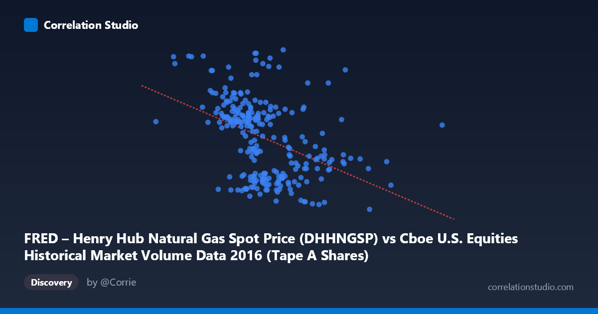
FRED – Henry Hub Natural Gas Spot Price (DHHNGSP) vs Cboe U.S. Equities Historical Market Volume Data 2016 (Tape A Shares)
- Pearson correlation (r)
- -0.425
- Spearman correlation
- -0.4599
- p-value
- 0
- Sample size (n)
- 252
- 95% confidence interval
- -0.5212 to -0.3182
- Granger causality
- None
- Granger optimal lag
- 1
AI analysis
Analysis: Henry Hub Natural Gas Spot Price vs. Cboe U.S. Equities Market Volume (2016)
Relationship Overview The scatterplot reveals a modest negative relationship between U.S. equities market trading volume (X-axis) and Henry Hub natural gas spot prices (Y-axis) across 252 paired daily observations spanning 2016. The linear regression equation (y = -4.057E-09x + 3.623) indicates that as equity market volume increases, natural gas spot prices tend to decline slightly. Visually, the data points form a diffuse, broadly scattered cloud with a gentle downward slope, suggesting the relationship — while statistically detectable — is far from deterministic. The two variables occupy very different scales and domains, making the apparent co-movement noteworthy but immediately inviting skepticism about underlying mechanisms.
Correlation Strength and Statistical Significance The Pearson correlation of r = -0.425 reflects a weak-to-moderate negative association, but the more informative metric is r² = 0.181, meaning only 18.1% of the variance in natural gas prices is explained by equity trading volume. Over 80% of the variation in gas prices is attributable to other factors entirely. The 95% confidence interval of [-0.521, -0.318] is reasonably tight and does not cross zero, and the p-value of 1.78E-12 confirms the correlation is highly statistically significant — almost certainly not a chance artifact given n = 252. However, statistical significance here is partly a function of the large population (N = 3,622); significance does not imply practical or economic meaningfulness. Crucially, Granger causality tests in both directions fail to reach significance (X→Y: F = 0.44, p = 0.51; Y→X: F = 0.11, p = 0.74), meaning neither variable temporally predicts the other at the tested lag. This effectively rules out a straightforward directional causal mechanism at the one-period lag tested.
Notable Patterns, Clusters, and Outliers Several features stand out in the sample points. The data cluster most densely in the X-range of roughly 220M–310M shares, which corresponds to typical daily equity volume in 2016, with natural gas prices scattered between approximately $1.77 and $3.06/MMBtu in that range. There are visible high-gas-price outliers at lower volume levels — notably the point near (190M, $3.50) and (278M, $3.56), which suggest that the highest gas prices occurred on relatively lower-volume equity days, consistent with the negative slope. The point cluster at lower X values (below ~230M shares) tends to show elevated Y values (gas prices above $2.70–$3.50), while higher-volume days (above ~300M shares) cluster more tightly around lower gas prices ($1.77–$2.30). This pattern loosely aligns with known seasonal effects in both markets during 2016.
Confounding Factors and Caveats This correlation almost certainly reflects shared seasonal confounding rather than any direct economic linkage. Natural gas prices in 2016 were heavily driven by weather patterns, storage levels, and LNG export dynamics — factors that push prices higher in winter months. Equity market volume, meanwhile, tends to be lower in summer months and during holiday-adjacent periods, and higher during periods of market volatility or institutional activity. If gas prices are high in winter (low-volume equity periods) and low in summer (higher-volume periods), a spurious negative correlation would emerge mechanically. The complete absence of Granger causality in either direction strongly reinforces that there is no economically meaningful lead-lag relationship. Additionally, the datasets appear to have been matched by date across entirely different domains ("Cboe U.S. Equities" and "FRED Henry Hub"), and the axis labels suggest a possible dataset column-to-dataset mismatch in labeling, warranting careful verification of the data join.
Actionable Insights and Further Investigation Given the absence of Granger causality and the relatively low r², this correlation should not be used as a predictive or trading signal in its current form. However, several follow-up analyses are warranted: (1) Deseasonalize both series using standard time-series decomposition to test whether the correlation persists after removing shared calendar effects — if it disappears, the seasonal confound explanation is confirmed; (2) Test multiple lags (beyond lag-1) in Granger causality, as energy-equity relationships sometimes operate over weekly or monthly horizons; (3) Segment by market regime — examine whether the correlation strengthens during periods of energy-sector volatility or broad market stress, when commodity and equity dynamics might genuinely interact; (4) Introduce control variables such as temperature anomalies, VIX levels, or energy sector ETF flows to isolate any residual relationship; and (5) verify the integrity of the data pairing, as the axis label descriptions appear inverted between dataset sources, which could affect interpretation of directionality entirely.
X dataset: Cboe U.S. Equities Historical Market Volume Data 2016
Y dataset: FRED – Henry Hub Natural Gas Spot Price
Part of experiment: Daily - Cboe U.S. Equities Historical Market Volume Data 2016 vs FRED – Henry Hub Natural Gas Spot Price