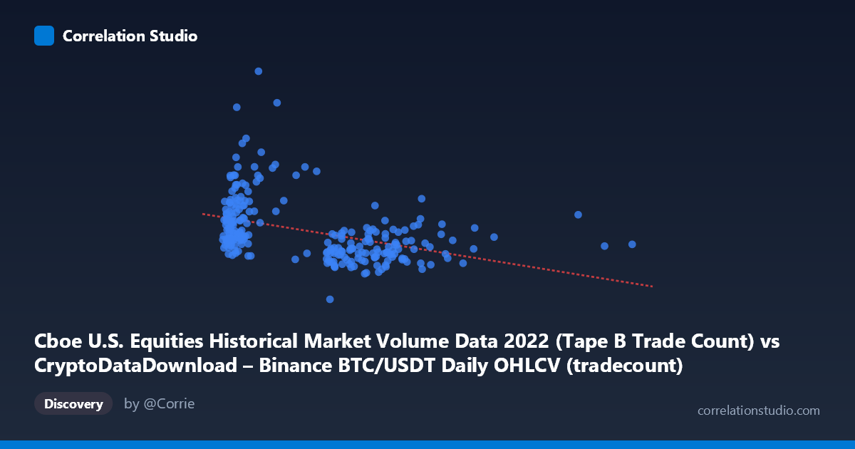
Cboe U.S. Equities Historical Market Volume Data 2022 (Tape B Trade Count) vs CryptoDataDownload – Binance BTC/USDT Daily OHLCV (tradecount)
- Pearson correlation (r)
- -0.4149
- Spearman correlation
- -0.4534
- p-value
- 0
- Sample size (n)
- 251
- 95% confidence interval
- -0.5124 to -0.3068
- Granger causality
- X → Y
- Granger optimal lag
- 10
- Time coverage
- 2022-01-03 to 2022-12-30
AI analysis
Analysis of the Relationship Between Cboe Trade Count and Binance BTC/USDT Trade Count
1. Overview of the Relationship
The scatterplot reveals a moderate negative, downward-sloping relationship between the two variables — as one column's trade count increases, the other tends to decrease. However, the data cloud is diffuse rather than tightly banded around the regression line, indicating substantial scatter and limiting confidence in the linear fit itself. The majority of points cluster in the lower-left-to-middle region of the X range (roughly 800,000–2,000,000), with a long, sparse tail of high-X observations extending out to ~14.5 million. This asymmetric distribution suggests the relationship is disproportionately influenced by a small number of high-leverage points.
2. Strength, Direction, and Statistical Confidence
The correlation coefficient (r = -0.4149) indicates a moderate negative relationship, but r² = 0.1721 tells the more important story: only about 17% of the variance in Y is explained by X, leaving over 80% attributable to other factors or noise. The 95% CI [-0.5124, -0.3068] is reasonably tight and entirely negative, and the p-value (7.29×10⁻¹²) confirms the correlation is highly statistically significant — this is not a spurious result of sampling noise. That said, statistical significance and practical significance diverge here: the relationship is real but weak in explanatory power.
The Granger causality results add a temporal dimension: X (Cboe trade count) appears to Granger-cause Y (Binance trade count) at a 10-period lag (F = 1.9067, p = 0.0454), while the reverse direction is not significant (p = 0.4046). This suggests a unidirectional, lagged predictive relationship — past Cboe equity trade activity may help forecast future Binance BTC/USDT activity, though the effect is only marginally significant (p just under 0.05) and the F-statistic is modest, warranting caution against overinterpretation.
3. Patterns, Clusters, and Outliers
Several notable features stand out: - A dense cluster of points with X between ~800K–2M and Y between ~400K–700K forms the core of the distribution. - A subset of points with unusually high Y values (e.g., ~940,000–1,212,000) sit within the low-X cluster, appearing as vertical outliers that don't follow the general downward trend — these likely correspond to specific high-volatility trading days. - As X increases beyond ~4M, Y values compress into a narrower band (~340,000–560,000), suggesting a possible non-linear (asymptotic or logarithmic) decay rather than a strictly linear relationship — the slope appears steeper at low X and flatter at high X. - The extreme X outliers (8M, up to 14.5M) are few in number but exert significant leverage on the regression slope.
4. Confounding Factors and Caveats
This is a cross-market, cross-asset comparison (traditional U.S. equities vs. a crypto exchange), so any correlation likely reflects shared macro drivers rather than direct mechanistic linkage. Both trade-count series are probably driven by common latent factors — overall market volatility, risk-on/risk-off sentiment, macroeconomic news cycles (Fed announcements, CPI releases), and calendar effects (weekday/weekend, holidays) — rather than one market directly causing activity in the other. Additionally, both series are time series with likely autocorrelation and potential trends/seasonality, which can inflate apparent correlation and complicate Granger causality interpretation (spurious regression risk). The small sample size (n=251 paired points from N=3,212) and unequal variance in X (huge range/stdev vs. Y) also mean the linear model is sensitive to the sparse high-X tail.
5. Suggestions for Further Investigation
- Detrend and de-seasonalize both series (e.g., differencing, removing day-of-week effects) before re-running correlation and Granger tests to rule out spurious relationships driven by shared trends. - Test a log-transform of X given its heavy right-skew and the apparent non-linear flattening at high values — this may improve model fit and better reveal the true functional form. - Investigate the high-Y outliers in the low-X cluster (dates with Y 900K) to identify specific market events (e.g., FTX collapse in Nov 2022) that may be driving disproportionate influence. - Include a third variable — such as a common volatility index (e.g., VIX or BTC realized volatility) — as a control to test whether the X-Y correlation persists or disappears, which would help distinguish genuine cross-market linkage from shared confounding drivers. - Given the marginal Granger p-value (0.0454), validate robustness with alternative lag structures and out-of-sample forecasting tests before relying on this for any predictive trading strategy.
X dataset: CryptoDataDownload – Binance BTC/USDT Daily OHLCV
Y dataset: Cboe U.S. Equities Historical Market Volume Data 2022
Part of experiment: Bitcoin - CryptoDataDownload – Binance BTC/USDT Daily OHLCV vs Cboe U.S. Equities Historical Market Volume Data 2022