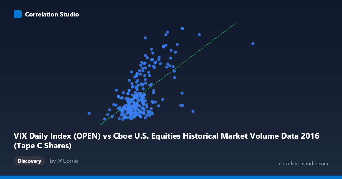
VIX Daily Index (OPEN) vs Cboe U.S. Equities Historical Market Volume Data 2016 (Tape C Shares)
- Pearson correlation (r)
- 0.6076
- Spearman correlation
- 0.5172
- p-value
- 0
- Sample size (n)
- 252
- 95% confidence interval
- 0.5233 to 0.6801
- Granger causality
- None
- Granger optimal lag
- 1
AI analysis
Scatterplot Analysis: VIX Daily Index (OPEN) vs. Tape C Shares (2016)
Overall Relationship The scatterplot reveals a moderate positive relationship between the VIX Daily Index opening values and Cboe U.S. Equities Tape C share volume across 2016. As VIX levels rise — reflecting increasing market fear or uncertainty — Tape C trading volume tends to increase as well. This is an intuitive and well-documented market dynamic: heightened volatility typically drives more active trading behavior, as investors rebalance portfolios, hedge positions, or react to news events. The linear regression equation (y = 9.04×10⁻⁸x + 3.99) confirms a positive slope, with the intercept suggesting a baseline volume level even at minimal volatility.
Correlation Strength and Statistical Significance The Pearson correlation of r = 0.608 indicates a moderate positive association, but the coefficient of determination r² = 0.369 is the more practically meaningful figure — it tells us that only about 36.9% of the variance in Tape C share volume is explained by VIX open levels. That leaves over 63% of variance attributable to other factors. The 95% confidence interval of [0.523, 0.680] is reasonably tight and does not cross zero, and the p-value of effectively 0 confirms this is not a chance finding in a sample of n = 252 drawn from a population of N = 3,622. However, the Granger causality tests tell a critically different story: neither direction (X→Y: F = 0.026, p = 0.871; Y→X: F = 0.059, p = 0.808) achieves significance at any conventional threshold. This means that despite the meaningful contemporaneous correlation, VIX does not temporally predict Tape C volume, nor vice versa — they move together without a clear lead-lag relationship at a 1-period lag.
Patterns, Clusters, and Outliers The sample points reveal notable structural features. The bulk of observations cluster in the X range of roughly 100–145 million with Y values between 12 and 18, forming a relatively dense core. However, there are clear high-leverage outliers at elevated VIX levels — most notably the point near (175M, 27.79) and another near (145M, 23.30) — which appear to exert considerable influence on the regression line and inflate the correlation coefficient. A point at approximately (166M, 22.15) similarly sits apart from the main cluster. Conversely, several high-X observations (e.g., ~163M, 13.94) show surprisingly low Y values, suggesting the relationship is heteroscedastic, with variance in Tape C shares increasing substantially at higher VIX levels. This fan-shaped spread undermines the assumptions of simple linear regression.
Confounding Factors and Caveats Several important caveats apply. First, the axes appear swapped from convention: VIX is typically treated as the independent market indicator, yet it appears on the X-axis while Tape C volume is on the Y-axis — this labeling should be verified to ensure correct interpretation. Second, 2016 was a historically eventful year (Brexit, U.S. presidential election), meaning a handful of high-volatility episodes may be driving the correlation disproportionately; the relationship in calmer periods may be much weaker. Third, Tape C volume (NYSE Arca-listed securities) is only one segment of total market volume, and routing decisions, market structure changes, and ETF activity could independently influence it. Fourth, both series likely share common latent drivers — macro uncertainty, institutional risk appetite, options expiration cycles — making it difficult to attribute causality even directionally.
Actionable Insights and Further Investigation Given the moderate correlation but absent Granger causality, practitioners should avoid using VIX as a short-term predictive signal for Tape C volume (or vice versa) in algorithmic or operational models. Instead, the relationship is better understood as contemporaneous co-movement driven by shared market conditions. Recommended next steps include: (1) testing non-linear models (e.g., log-log or polynomial regression) to better capture the apparent heteroscedasticity; (2) segmenting the data by volatility regime (low/medium/high VIX) to assess whether the relationship strengthens at extreme values; (3) extending Granger tests to longer lags (2–5 periods) to rule out delayed predictive effects; and (4) including additional covariates such as S&P 500 returns, options volume, or total market volume to build a more complete explanatory model.
X dataset: Cboe U.S. Equities Historical Market Volume Data 2016
Y dataset: VIX Daily Index
Part of experiment: Daily - Cboe U.S. Equities Historical Market Volume Data 2016 vs VIX Daily Index