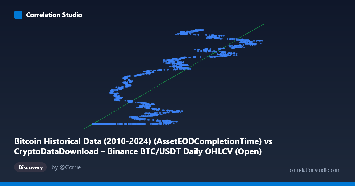
Bitcoin Historical Data (2010-2024) (AssetEODCompletionTime) vs CryptoDataDownload – Binance BTC/USDT Daily OHLCV (Open)
- Pearson correlation (r)
- 0.8518
- Spearman correlation
- 0.8876
- p-value
- 0
- Sample size (n)
- 3191
- 95% confidence interval
- 0.842 to 0.8611
- Granger causality
- None
- Granger optimal lag
- 10
AI analysis
Analysis: Bitcoin Timestamp vs. Price Relationship
What the Visualization Reveals
This scatterplot is somewhat unusual in that the X-axis variable is described as a timestamp/completion-time field rather than a conventional independent variable, while Y is BTC/USDT opening price. Given the sample points, X appears to behave more like a row-index or sequence-derived numeric value (ranging ~3,188 to ~124,658) that correlates with the chronological progression of the dataset, rather than a raw Unix timestamp. Practically, this means the chart is really showing Bitcoin's price trajectory over sequential time, with clusters at the low end of X (~3,000–20,000) tightly bunched near the $1.614B mark (likely representing early low-price periods, possibly index/legacy scaling), while higher X values spread out substantially toward $1.7–1.78B, corresponding to bull-market price appreciation.
Strength, Direction, and Uncertainty
The correlation is strong and positive (r = 0.852), with R² = 0.726 indicating that roughly 73% of the variance in Y is explained by X in a linear framework — a substantial but not complete explanatory relationship. The tight 95% CI [0.842, 0.861] and p-value of ~0 confirm this relationship is highly statistically reliable and not a product of sampling noise, given the large n (3,191). However, statistical significance here reflects the strength of the pattern in-sample, not causal proof. Critically, the Granger causality tests show no significant predictive direction in either direction (X→Y: p=0.33; Y→X: p=0.15). This is an important caveat: despite the strong contemporaneous correlation, neither variable helps forecast the other's future values beyond its own history at the tested lag (10 periods). This strongly suggests the relationship is driven by a shared underlying trend (time itself, or market-wide bull momentum) rather than one variable mechanically leading the other.
Notable Patterns and Non-linearities
The data is not uniformly linear — sample points reveal a distinct "floor" cluster where X < ~20,000 corresponds almost invariably to Y ≈ 1,614,337,xxx (an oddly constant value with minimal variance), suggesting a data artifact, a price floor/support period, or an anomalous encoding for early records. Beyond this cluster, Y increases with X but with considerable dispersion and volatility (e.g., X=57,635 → Y=1.617B vs. X=57,037 → Y=1.709B), indicating heteroscedasticity — variance in Y grows substantially at mid-to-high X values. This is consistent with crypto markets' well-known volatility clustering and suggests the true relationship may be better modeled as piecewise, logarithmic, or with regime-switching components rather than a single linear fit.
Confounding Factors and Caveats
Several caveats apply: (1) The X variable's true meaning is ambiguous — if it's a transformed/scaled timestamp or row index, the "correlation" is essentially a proxy for time-trend, which is not informative about market mechanics per se. (2) Bitcoin prices are non-stationary and trend-driven, so classic Pearson correlation and linear R² can be inflated by shared trend components — a spurious regression risk common in time-series economics. (3) The flat cluster at low X values (identical Y across many rows) suggests possible data quality issues, padding, or repeated/missing values from an early period that should be scrutinized before drawing conclusions. (4) Macro factors (halving cycles, regulatory news, exchange-specific liquidity events) are omitted from this bivariate analysis and likely drive much of the unexplained ~27% variance.
Actionable Insights
1. Verify the X variable's construction — confirm whether it's a raw timestamp, transformed timestamp, or index, since this fundamentally changes interpretation. 2. Investigate the low-X flat cluster for data quality issues (duplicate entries, placeholder values, or a genuine low-volatility historical period). 3. De-trend or difference both series before further correlation/causality testing to mitigate spurious trend-driven correlation — consider log returns instead of levels. 4. Explore non-linear/piecewise models (e.g., log-linear, spline regression) given evident heteroscedasticity and clustering. 5. Given the null Granger result, avoid using this relationship for predictive trading models; instead, treat it as descriptive of historical trend alignment only.
X dataset: CryptoDataDownload – Binance BTC/USDT Daily OHLCV
Y dataset: Bitcoin Historical Data (2010-2024)
Part of experiment: Bitcoin - CryptoDataDownload – Binance BTC/USDT Daily OHLCV vs Bitcoin Historical Data (2010-2024)