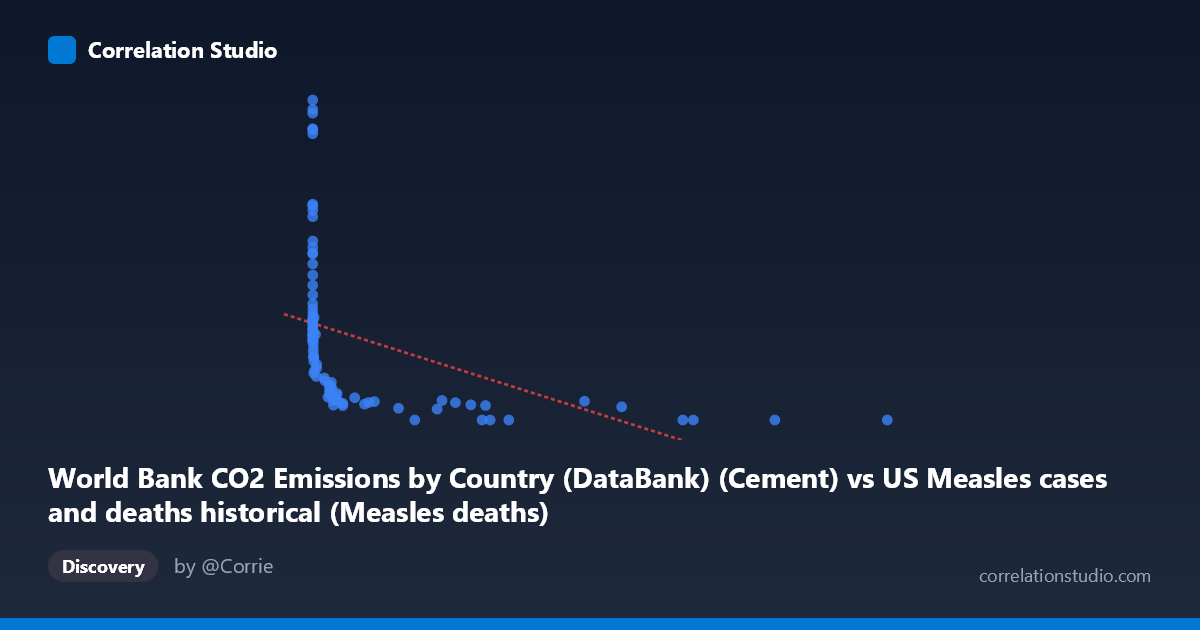
World Bank CO2 Emissions by Country (DataBank) (Cement) vs US Measles cases and deaths historical (Measles deaths)
- Pearson correlation (r)
- -0.4227
- Spearman correlation
- -0.9456
- p-value
- 0.000027
- Sample size (n)
- 92
- 95% confidence interval
- -0.5776 to -0.2386
- Granger causality
- None
- Granger optimal lag
- 10
AI analysis
Analysis: Cement CO2 Emissions vs. US Measles Deaths (1919–2020)
1. What the Visualization Reveals
The scatterplot displays a weak-to-moderate negative relationship between global cement CO2 emissions and US measles deaths across roughly a century of annual observations. The most immediately striking visual feature is the L-shaped or hyperbolic distribution of points: measles deaths cluster at very high values (700–2600) when cement emissions are near zero, while at higher emission values, deaths collapse toward zero. This pattern visually dominates the chart and immediately suggests that a simple linear model is a poor description of the underlying structure — the relationship is fundamentally non-linear, with deaths declining steeply at first and then flattening.
2. Correlation Strength, Direction, and Causality
The Pearson correlation of r = −0.4227 indicates a moderate negative association, but the R² of 0.179 means that cement CO2 emissions explain only 17.9% of the variance in US measles deaths — leaving over 82% unexplained by this variable alone. The 95% confidence interval of [−0.578, −0.239] confirms the effect is statistically distinguishable from zero (p = 2.7×10⁻⁵), but the width of that interval reflects meaningful uncertainty about the true effect size. Critically, the Granger causality analysis finds no significant predictive direction in either direction (X→Y: F = 0.89, p = 0.55; Y→X: F = 0.95, p = 0.50), meaning that past values of cement emissions do not help forecast measles deaths, and vice versa. This is a strong signal that the observed correlation, while statistically real, likely reflects shared temporal trends rather than any mechanistic or causal pathway. The note that Spearman ρ exceeds Pearson r further confirms that the monotonic but non-linear structure is being partially missed by the linear model.
3. Notable Patterns, Clusters, and Outliers
Several structural features stand out:
- High-leverage outliers at extreme X values: Points like (12,992; 0), (10,450; 0), and (8,607; 0) anchor the negative slope but represent late-20th-century years when measles was effectively eliminated in the US — these points are influential in pulling down the regression line. - High-Y, near-zero-X cluster: Many points with X ≈ 0–50 show Y values ranging from ~500 to over 2,600 deaths, representing pre-1940s observations when industrial cement production was minimal and measles was endemic. - One notable outlier: The point (1; 2,532.94) and (0; 2,608.93) represent exceptionally high death years, likely epidemic peaks in the 1920s–1930s. - Middle-range compression: Points with X between ~300–1,500 show moderate Y values (100–450), consistent with the post-WWII transition period when vaccines were not yet available but public health improvements had begun reducing mortality.
4. Confounding Factors and Interpretive Caveats
The correlation almost certainly reflects nothing more than two independent secular trends across the 20th century: measles deaths declined due to vaccination (1963), improved medical care, and public health infrastructure, while cement CO2 emissions rose due to global industrialization and population growth. These trends happen to move in opposite directions over time, producing a spurious negative correlation — a textbook case of confounding by time. Additional caveats include: (1) the datasets come from entirely different domains (global industrial emissions vs. US epidemiology), making any direct mechanism implausible; (2) the X variable is global cement emissions, not US-specific, adding further ecological mismatch; (3) the zero-inflated nature of both variables in different eras creates heteroscedasticity that violates linear regression assumptions; and (4) the optimal lag of 10 periods in the Granger test, combined with non-significant results, suggests no temporal structure links these series even at extended horizons.
5. Actionable Insights and Further Investigation
Given that this correlation is almost certainly spurious, the primary analytical value here is methodological illustration rather than substantive insight. Recommended next steps include: (1) detrending both time series (e.g., first-differencing or regressing out year) before computing correlations, to test whether any residual association survives removal of shared secular trends; (2) fitting a logarithmic or power-law model given the strong non-linearity suggested by the L-shaped scatter — this would better characterize the distributional shape even if causality remains absent; (3) segmenting the analysis by era (pre-vaccine pre-1963 vs. post-vaccine) to test whether the correlation structure differs meaningfully; and (4) if the substantive goal is understanding measles mortality drivers, replacing cement emissions with variables like vaccination coverage rates, healthcare access indices, or population density that have plausible biological mechanisms. The Granger non-result is actually the most important finding here — it closes the door on any predictive utility of this pairing.
X dataset: US Measles cases and deaths historical
Y dataset: World Bank CO2 Emissions by Country (DataBank)
Part of experiment: Yearly - US Measles cases and deaths historical vs World Bank CO2 Emissions by Country (DataBank)