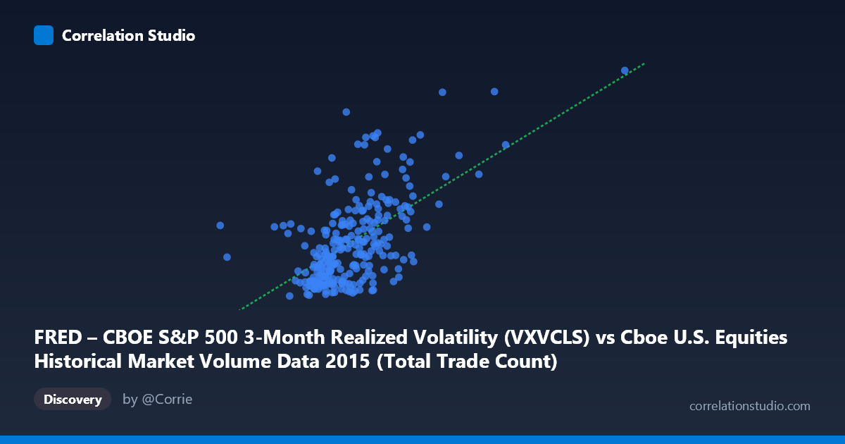
FRED – CBOE S&P 500 3-Month Realized Volatility (VXVCLS) vs Cboe U.S. Equities Historical Market Volume Data 2015 (Total Trade Count)
- Pearson correlation (r)
- 0.5816
- Spearman correlation
- 0.5338
- p-value
- 0
- Sample size (n)
- 252
- 95% confidence interval
- 0.4935 to 0.6579
- Granger causality
- None
- Granger optimal lag
- 1
AI analysis
Analysis: CBOE S&P 500 3-Month Realized Volatility vs. Total Trade Count (2015)
Relationship Overview The scatterplot reveals a moderate positive relationship between the CBOE S&P 500 3-Month Realized Volatility (VXVCLS) on the X-axis and the Total Trade Count on the Y-axis across U.S. equity markets in 2015. As realized volatility increases, total trade count tends to rise, which aligns intuitively with market microstructure theory: higher volatility environments typically generate more frequent trading activity as participants react to price uncertainty, rebalance positions, and execute hedging strategies. The linear regression equation (y = 4.00397E-06x + 8.55148) confirms this positive slope, though the relationship is far from deterministic.
Correlation Strength and Statistical Significance The Pearson correlation of r = 0.5816 indicates a moderate positive association, but the explanatory power is more sobering when framed through r²: only 33.8% of the variance in trade count is explained by realized volatility, leaving roughly two-thirds attributable to other factors. The 95% confidence interval of [0.4935, 0.6579] is reasonably tight given the sample size of n = 252, and the p-value of effectively zero confirms this relationship is highly unlikely to be a statistical artifact. However, the Granger causality results tell a critical story: neither direction (X→Y: F = 0.0085, p = 0.9266; Y→X: F = 0.1865, p = 0.6662) achieves significance, meaning that past values of realized volatility do not reliably predict future trade counts, and vice versa. The contemporaneous correlation is real, but it carries no demonstrated temporal predictive power at a one-period lag.
Patterns, Clusters, and Outliers Several notable structural features emerge from the sample points. The bulk of observations cluster in the X range of roughly 1.8M–2.8M with Y values between 14 and 22, forming a dense core that anchors the regression line. However, there are clear high-leverage outliers in the upper-right quadrant — most strikingly the point near (4,083,022, 29.58) and another near (3,907,921, 23.47) — which likely correspond to the pronounced volatility spike during the August 2015 market selloff, when equity markets experienced sharp drawdowns and trading volumes surged simultaneously. The point at (997,371, 19.69) stands out as an anomalous low-volume day with moderate volatility, potentially a holiday-shortened session. There also appears to be a heteroscedastic fan shape, where variance in trade counts expands considerably at higher volatility levels, suggesting the relationship is not uniformly linear across the full range.
Confounding Factors and Caveats Several confounds warrant caution. First, both variables are likely driven by common underlying market stress factors — such as macroeconomic announcements, Federal Reserve communications, or geopolitical events — making it difficult to attribute directional causality. Second, the 3-month realized volatility measure is backward-looking by construction, which partially explains the absence of Granger causality; it smooths over daily fluctuations that drive intraday trading decisions. Third, market structure changes within 2015 (e.g., shifts in algorithmic trading, exchange fee schedules, or regulatory events) could introduce non-stationarity that inflates the apparent correlation. Finally, the dataset covers only a single calendar year, limiting generalizability, and the N = 3,302 population versus n = 252 sample suggests the paired observations represent a subset that may not fully capture the distribution's tails.
Actionable Insights and Further Investigation Practitioners should avoid using lagged realized volatility as a standalone predictor of trade count given the failed Granger causality tests — any trading or risk model relying on this signal for next-day volume forecasting would be poorly grounded. More productive next steps would include: (1) incorporating implied volatility (VIX) alongside realized volatility, as forward-looking measures may better capture the uncertainty that drives trading decisions; (2) segmenting the analysis by market regime (low-vol vs. high-vol periods) to test whether the correlation strengthens nonlinearly during stress events like August 2015; (3) applying a log transformation to the volume variable to address the apparent heteroscedasticity and potential multiplicative dynamics; and (4) extending the time series across multiple years to test whether the 2015 relationship is stable or regime-dependent, particularly given the outsized influence of the summer volatility episode on the current correlation estimate.
X dataset: Cboe U.S. Equities Historical Market Volume Data 2015
Y dataset: FRED – CBOE S&P 500 3-Month Realized Volatility
Part of experiment: Daily - Cboe U.S. Equities Historical Market Volume Data 2015 vs FRED – CBOE S&P 500 3-Month Realized Volatility