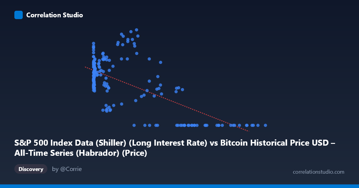
S&P 500 Index Data (Shiller) (Long Interest Rate) vs Bitcoin Historical Price USD – All-Time Series (Habrador) (Price)
- Pearson correlation (r)
- -0.6533
- Spearman correlation
- -0.4724
- p-value
- 0
- Sample size (n)
- 189
- 95% confidence interval
- -0.7281 to -0.563
- Granger causality
- Y → X
- Granger optimal lag
- 1
AI analysis
Analysis: Bitcoin Price vs. Long Interest Rate
Note on axis labeling: The column labels appear swapped relative to the described datasets — X is labeled as "Long Interest Rate" but ranges into six figures (0.06 to 118,670), consistent with Bitcoin price data, while Y (0–4.17) behaves like an interest rate. This analysis treats X as Bitcoin price and Y as the S&P/Shiller long interest rate, based on the actual data ranges.
1. What the Visualization Reveals
The scatterplot shows a clear negative, non-linear relationship. At low Bitcoin prices (under ~1,000), Y values cluster tightly between 1.6 and 3.6, showing considerable variability but no strong trend. As X increases into the tens of thousands, Y systematically collapses toward zero — nearly every observation above X ≈ 55,000 has Y = 0.00. This produces a curve that looks more like a threshold/decay function than a straight line.
2. Strength, Direction, and Statistical Confidence
The Pearson correlation of r = -0.6533 indicates a moderately strong negative linear association, with r² = 0.427 meaning Bitcoin price (or its proxy variable) explains about 43% of the variance in the rate variable — leaving the majority (57%) unexplained by this simple linear relationship. The 95% CI [-0.728, -0.563] is reasonably tight and excludes zero, and the p-value ≈ 0 confirms this relationship is highly unlikely to be due to chance. However, statistical significance here reflects the strong monotonic pattern (especially the "flatline at zero" behavior for high X), not necessarily a clean linear mechanism.
The Granger causality result is notable: Y Granger-causes X, not the reverse (F=4.87, p=0.0285 vs. F=0.83, p=0.365 for the opposite direction). This suggests that historical values of the rate variable have predictive power for future Bitcoin price movements, but Bitcoin price does not predict future rate changes. Practically, this hints that macro rate conditions may lead price action rather than the other way around — though with only 189 paired points against 1,865 total periods (~10% sampling), this should be treated as suggestive rather than conclusive.
3. Patterns, Clusters, and Outliers
Three distinct regimes are visible: - Low-X cluster (X < 1,000): Dense, scattered Y values (1.6–3.6), representing the vast majority of points — likely Bitcoin's early years when prices were low and rates fluctuated normally. - Mid-X transition (1,000–40,000): Y values decline gradually and grow more variable (0.87–4.17), including the single highest Y value (4.17) at X≈29,676 — an outlier suggesting rate spikes can co-occur with moderate Bitcoin prices. - High-X plateau (X 55,000): Y collapses almost uniformly to 0.00, an unnatural-looking floor effect that dominates the negative correlation and may reflect data censoring, a rate hitting a zero lower bound, or a structural break/regime change (e.g., a policy period) rather than a continuous economic relationship.
4. Confounding Factors and Caveats
The apparent "floor" at Y=0 for large X is suspicious — it may indicate missing/zero-filled data rather than a true economic rate of zero, which would artificially inflate the negative correlation. Both series are also strongly time-trending (Bitcoin price has grown exponentially over 2010–2026, while long rates followed their own multi-year cycle, e.g., declining post-2020 and rising after 2022), so the correlation may largely reflect spurious trend correlation rather than a direct causal link. Neither series is stationary, which can invalidate both the Pearson r and Granger test unless properly differenced.
5. Suggestions for Further Investigation
- Verify axis labels/data alignment — confirm which variable is truly X vs. Y given the mismatch between described column names and observed ranges. - Check the zero-Y values for high X: are these genuine zero rates or missing/placeholder data? - Log-transform Bitcoin price (given its multiple orders of magnitude range) and re-run correlation/regression to check if the relationship is better described as log-linear. - Difference or detrend both series before Granger testing to rule out spurious trend-driven causality. - Segment by time period (e.g., pre/post-2020) to see if the relationship is stable or driven by a specific macro regime (e.g., zero-rate era coinciding with Bitcoin's price run-up).
X dataset: Bitcoin Historical Price USD – All-Time Series (Habrador)
Y dataset: S&P 500 Index Data (Shiller)
Part of experiment: Bitcoin - Bitcoin Historical Price USD – All-Time Series (Habrador) vs S&P 500 Index Data (Shiller)