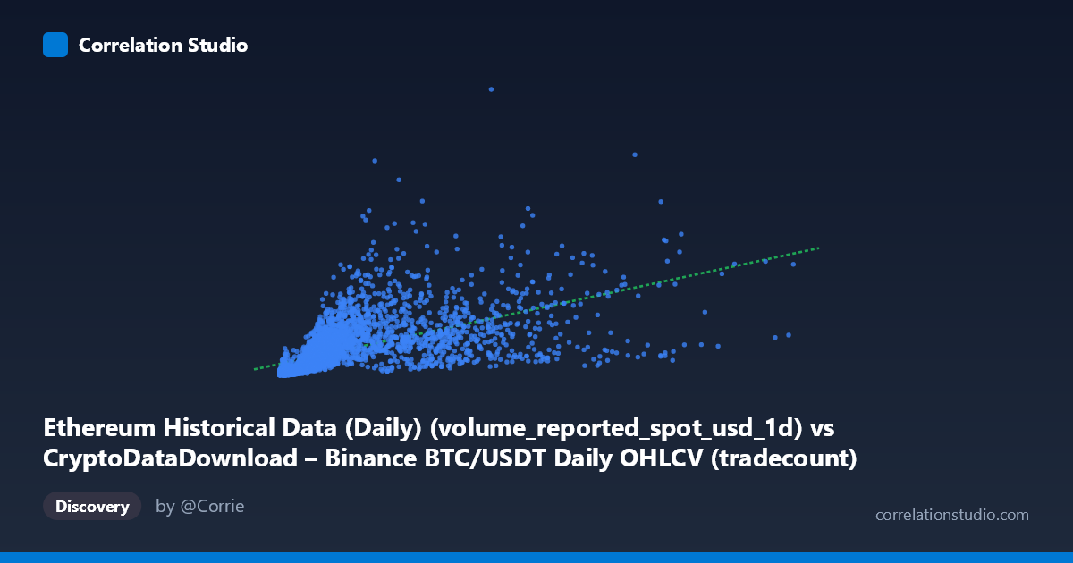
Ethereum Historical Data (Daily) (volume_reported_spot_usd_1d) vs CryptoDataDownload – Binance BTC/USDT Daily OHLCV (tradecount)
- Pearson correlation (r)
- 0.5837
- Spearman correlation
- 0.8324
- p-value
- 0
- Sample size (n)
- 3191
- 95% confidence interval
- 0.5603 to 0.6061
- Granger causality
- None
- Granger optimal lag
- 10
AI analysis
Analysis: Ethereum Volume vs. Bitcoin Trade Count Relationship
Note on labeling: The axis metadata appears mismatched (X labeled as Ethereum volume but described as BTC/USDT volume; Y labeled as BTC tradecount but described as Ethereum metrics). I'll analyze based on the actual data behavior: X is a volume-like metric (range 2K–15.3M, right-skewed) and Y is a count/activity metric (range 108M–53.7B) that scales positively with X.
1. Overall Relationship
The scatterplot shows a positive, moderate-strength association: as X increases, Y tends to increase as well, but the relationship is loose rather than tight. Data points form a widening cone/fan shape typical of heteroscedastic financial or on-chain data — variance in Y grows substantially as X increases, rather than points hugging a single line.
2. Strength, Direction, and Statistical Confidence
- Correlation (r = 0.584) indicates a moderate positive linear relationship. - r² = 0.341 means only ~34% of the variance in Y is explained by X — the majority (66%) is driven by other factors, noise, or nonlinear dynamics not captured by this simple linear model. - The 95% CI [0.560, 0.606] is fairly tight given the large sample (n=3,191), and the p-value ≈ 0 confirms the correlation is highly statistically significant — this relationship is not due to chance. - However, statistical significance ≠ practical strength: with r² only ~0.34, X alone is a weak-to-moderate predictor of Y in practice. - Granger causality tests show no significant predictive direction in either direction (X→Y: p=0.42; Y→X: p=0.18) at the optimal 10-period lag. This is important: despite the contemporaneous correlation, neither variable helps forecast the other's future values in a time-series sense. The relationship appears to be driven by shared contemporaneous market conditions (e.g., both responding to volatility, exchange activity, or broader crypto market cycles) rather than one causing/leading the other.
3. Patterns, Clusters, and Outliers
- The data is heavily right-skewed in X (mean 1.97M vs. median likely much lower, stdev 2.24M ≈ mean), with a dense cluster of low-X points and a long tail of large-volume days. - Several high-leverage outliers exist at high X (e.g., X≈8.7M→Y≈19B; X≈15.3M at the extreme) that could disproportionately influence the linear fit. - At low X values, Y still spans a wide range (e.g., X≈9,324 → Y≈204M, but X≈2,260 → Y≈272M, and X≈259,212 → Y≈2.05B), suggesting a non-linear or log-linear relationship — small increases in X near the origin correspond to large jumps in Y. - This is supported by the note that Spearman ρ exceeds Pearson r, indicating the true relationship is likely monotonic but curved (e.g., logarithmic, power-law) rather than strictly linear — consistent with typical volume/activity metrics in crypto markets which often follow power-law scaling.
4. Confounding Factors and Caveats
- Shared market regime effects: both variables likely respond to the same external drivers (bull/bear cycles, volatility spikes, macro news), creating spurious contemporaneous correlation without direct causal linkage — consistent with the null Granger result. - Scale mismatch and skewness: raw linear regression is likely a poor fit given the skewed distributions; log-transforming both variables before modeling would likely improve fit and interpretability. - Autocorrelation: daily financial/on-chain time series are typically autocorrelated, which can inflate apparent correlation and violate independence assumptions in significance testing (though p-value here is already near-zero, so this mainly affects effect-size interpretation, not significance). - Metadata inconsistency: the mismatched column descriptions raise data-integrity concerns — verify the actual source/definition of each variable before drawing domain conclusions.
5. Recommendations for Further Investigation
- Re-fit using log-log or log-linear regression to test whether a power-law/logarithmic model substantially improves R² — the Spearman/Pearson divergence strongly suggests this. - Decompose by time period/regime (e.g., bull vs. bear markets, halving cycles) to check if the relationship strength varies over time rather than being stable. - Control for a common confounder (e.g., overall market volatility index or total crypto market cap) via partial correlation to test if the X-Y link is genuinely direct or mediated. - Verify and correct axis labeling before publishing conclusions, given the metadata mismatch. - Given the null Granger result, do not use X as a leading indicator for Y (or vice versa) in forecasting models; treat the correlation as descriptive/contemporaneous only.
X dataset: CryptoDataDownload – Binance BTC/USDT Daily OHLCV
Y dataset: Ethereum Historical Data (Daily)
Part of experiment: Bitcoin - CryptoDataDownload – Binance BTC/USDT Daily OHLCV vs Ethereum Historical Data (Daily)