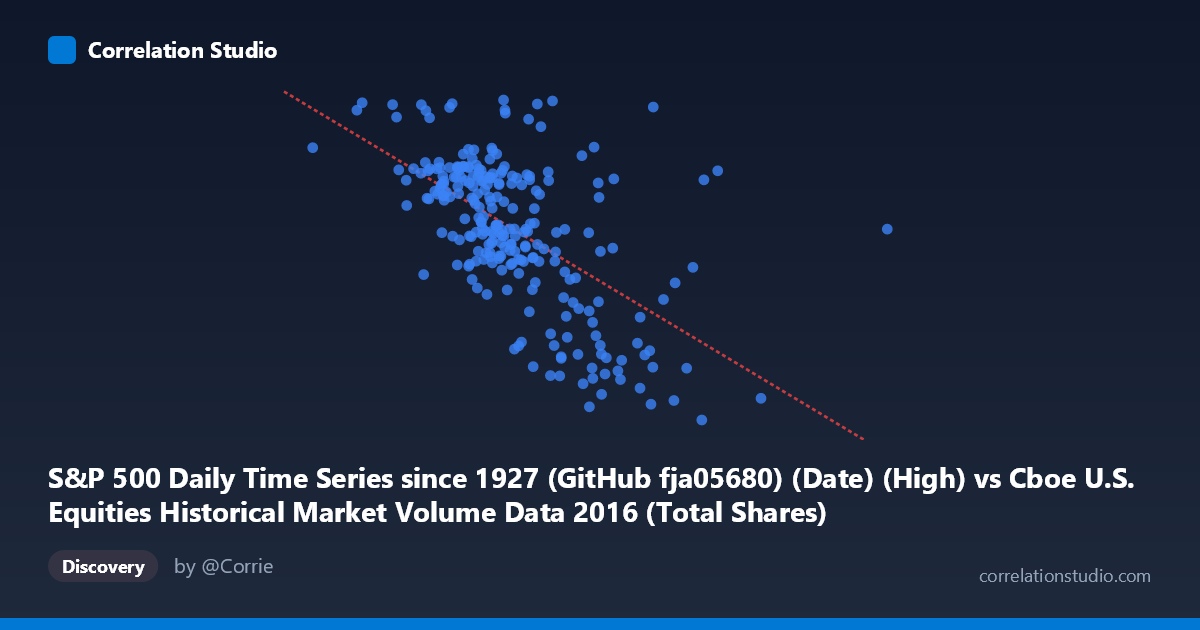
S&P 500 Daily Time Series since 1927 (GitHub fja05680) (Date) (High) vs Cboe U.S. Equities Historical Market Volume Data 2016 (Total Shares)
- Pearson correlation (r)
- -0.5911
- Spearman correlation
- -0.5821
- p-value
- 0
- Sample size (n)
- 252
- 95% confidence interval
- -0.666 to -0.5043
- Granger causality
- None
- Granger optimal lag
- 4
AI analysis
Analysis: S&P 500 Daily High vs. Total Shares Traded (2016)
Relationship Overview The scatterplot reveals a moderate negative relationship between the S&P 500 daily high price (X-axis) and the total shares traded on U.S. equities exchanges (Y-axis) across 2016. As the index reached higher price levels, total share volume tended to decline — a pattern that is visually apparent as a downward-sloping cloud of points. The linear regression equation (y = -5.20×10⁻⁷x + 2369.98) captures this inverse trend, though considerable scatter around the regression line indicates that price alone is far from a complete explanation of trading volume dynamics.
Correlation Strength and Statistical Significance The Pearson correlation of r = -0.5911 reflects a moderate negative association. The R² of 0.3494 means that roughly 35% of the variance in total shares traded is explained by the S&P 500 daily high — meaningful, but leaving 65% of variation attributable to other factors. The 95% confidence interval of [-0.6660, -0.5043] is entirely negative and reasonably tight given a paired sample of n = 252 drawn from a population of N = 3,622, and the p-value of essentially 0 confirms this is not a chance finding. However, the Granger causality results tell a more cautionary story: neither direction (X→Y nor Y→X) achieves significance at the optimal lag of 4 periods (F = 0.55, p = 0.70 for X→Y; F = 1.42, p = 0.23 for Y→X). This means that while the two variables are contemporaneously correlated, neither reliably predicts the other temporally — a critical distinction for anyone tempted to use price levels to forecast future volume or vice versa.
Patterns, Clusters, and Outliers Several notable features emerge from the point distribution. There is a visible dense cluster between approximately 420M–560M on the X-axis and 2,050–2,200 on the Y-axis, corresponding to the mid-range S&P 500 prices and moderate volume levels that dominated much of 2016. At the lower-left extremity (X values around 200–350M), a handful of high-volume observations appear (Y near 2,183–2,271), suggesting elevated share counts on days with lower index levels — likely corresponding to the market stress and volatility of early 2016. Conversely, high-X outliers (e.g., near 700M–1,092M) consistently show depressed Y values (around 1,847–1,920), consistent with a post-election or late-year rally environment where higher prices coincide with reduced share turnover. The point at approximately (549M, 2,272) stands out as an anomaly — unusually high volume for its price level — warranting individual date-level investigation.
Confounding Factors and Caveats Several important caveats apply. First, share price and share volume have a mechanical inverse relationship: as index prices rise over time, the same notional dollar volume corresponds to fewer shares traded, creating a structural bias toward negative correlation that may not reflect genuine investor behavior changes. Second, 2016 was an atypical year with distinct volatility regimes — early-year turbulence, Brexit (June), and the U.S. election (November) — meaning the correlation may be driven partly by regime clustering rather than a stable underlying mechanism. Third, the datasets originate from different sources (Cboe market volume vs. Yahoo Finance S&P 500 prices), introducing potential alignment or measurement inconsistencies. Finally, the absence of Granger causality suggests the correlation is largely contemporaneous and possibly spurious — driven by shared macroeconomic conditions rather than a direct price-volume transmission mechanism.
Actionable Insights and Further Investigation Practitioners should avoid using S&P 500 price levels alone as a forward-looking volume predictor, given the failed Granger causality tests. A more productive investigation would involve: (1) normalizing share volume to notional dollar volume to remove the mechanical price-per-share effect and test whether any genuine behavioral relationship persists; (2) segmenting by volatility regime (e.g., using VIX thresholds) to assess whether the correlation strengthens during stress periods; (3) extending the time horizon beyond 2016 to test stability of this relationship across bull and bear markets; and (4) including additional predictors such as bid-ask spreads, VIX levels, or options volume to build a more complete model of the 65% unexplained variance. The outlier near (549M, 2,272) should be examined individually to determine whether it reflects a data anomaly or a genuine event-driven volume spike.
X dataset: Cboe U.S. Equities Historical Market Volume Data 2016
Y dataset: S&P 500 Daily Time Series since 1927 (GitHub fja05680) (Date)
Part of experiment: Daily - Cboe U.S. Equities Historical Market Volume Data 2016 vs S&P 500 Daily Time Series since 1927 (GitHub fja05680) (Date)