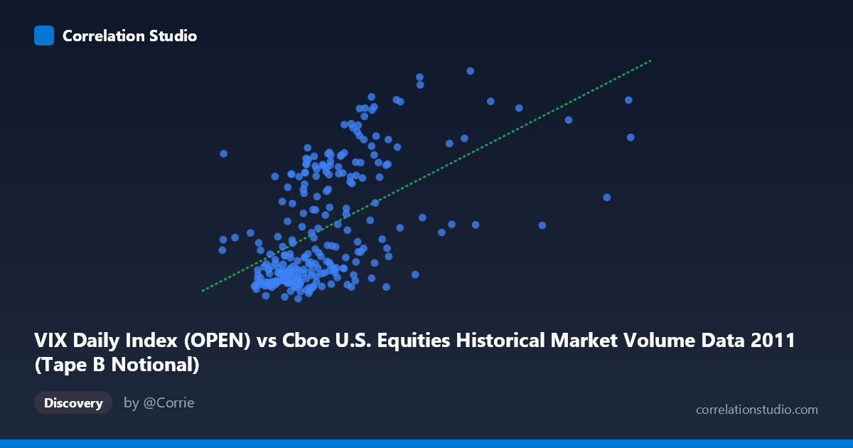
VIX Daily Index (OPEN) vs Cboe U.S. Equities Historical Market Volume Data 2011 (Tape B Notional)
- Pearson correlation (r)
- 0.5378
- Spearman correlation
- 0.5706
- p-value
- 0
- Sample size (n)
- 252
- 95% confidence interval
- 0.4438 to 0.6202
- Granger causality
- None
- Granger optimal lag
- 1
AI analysis
Scatterplot Analysis: VIX Open vs. Tape B Notional Volume (2011)
Overall Relationship The scatterplot reveals a moderate positive relationship between the VIX Daily Index opening values and Tape B Notional trading volume across U.S. equities exchanges in 2011. As VIX levels rise — indicating heightened market fear or uncertainty — Tape B Notional volume tends to increase as well. This is an intuitively plausible connection: periods of elevated volatility typically drive greater trading activity as market participants reposition, hedge, or react to rapidly changing conditions. The linear regression equation (y = 2.45×10⁻⁹x + 11.77) confirms the positive slope, though the relationship is far from deterministic.
Correlation Strength and Statistical Framing The Pearson correlation of r = 0.538 indicates a moderate positive association, but the coefficient of determination (r² = 0.289) is the more sobering figure — only 28.9% of the variance in Tape B Notional volume is explained by VIX Open levels, leaving roughly 71% attributable to other factors. The 95% confidence interval for r spans [0.44, 0.62], which is meaningfully wide, suggesting non-trivial uncertainty in the true population relationship despite the statistically significant p-value (~0) derived from a population size of N = 3,780. Critically, the Granger causality tests show no significant predictive directionality in either direction (X→Y: F = 0.223, p = 0.637; Y→X: F = 0.038, p = 0.846). This means that even though the two variables co-move, knowing today's VIX does not meaningfully improve predictions of tomorrow's Tape B volume, and vice versa — the relationship is contemporaneous rather than temporally predictive.
Notable Patterns, Clusters, and Outliers The scatterplot data reveals several distinct features worth noting. There appears to be a dense cluster of observations concentrated in the lower-left region, where VIX values fall below ~22 and Tape B Notional volume clusters near the lower range — consistent with calmer market periods in early 2011. A secondary, more dispersed cluster appears at higher VIX levels (roughly 30–46), corresponding to the elevated volatility environment of mid-to-late 2011 during the European sovereign debt crisis and the U.S. debt ceiling debate. Several notable outliers stand out, including the point near (9,956M, 41.94) and (6,103M, 40.93), which represent extreme combinations of both high volatility and high notional volume. The scatter also appears to fan outward at higher X values, hinting at possible heteroscedasticity — variance in Tape B volume increases as VIX rises, which violates a key assumption of ordinary least squares regression.
Confounding Factors and Caveats Several important caveats temper interpretation. First, the axes appear to be swapped relative to conventional expectation: VIX is plotted on the X-axis while Tape B Notional volume occupies the Y-axis, yet VIX is typically considered the independent market signal — users should verify column assignments are intentional. Second, both variables are likely driven by common macroeconomic shocks (e.g., the August 2011 S&P downgrade of U.S. debt, Eurozone headlines), meaning the correlation may reflect shared external forcing rather than any direct causal link. Third, the lack of Granger causality at lag 1 suggests the relationship is largely synchronous, potentially an artifact of within-day or event-driven dynamics not well-captured by daily data. Finally, Tape B specifically covers NYSE American and regional exchange stocks, which may behave differently from the broader market VIX measures.
Actionable Insights and Further Investigation Practitioners should avoid using VIX alone as a predictive tool for Tape B Notional volume given the weak Granger causality results — the relationship is better characterized as a concurrent indicator than a leading one. Recommended next steps include: (1) testing non-linear models (e.g., polynomial or spline regression) to better capture the apparent heteroscedasticity and possible threshold effects above VIX = 30; (2) segmenting the data by market regime (pre- and post-August 2011 debt crisis) to examine whether the correlation strengthens in high-stress periods; (3) incorporating additional explanatory variables such as overall market breadth, macroeconomic announcements, or Tape A/C volumes to build a more complete model of volume behavior; and (4) extending the analysis across multiple years to determine whether this moderate correlation is stable or specific to the unique volatility environment of 2011.
X dataset: Cboe U.S. Equities Historical Market Volume Data 2011
Y dataset: VIX Daily Index
Part of experiment: Daily - Cboe U.S. Equities Historical Market Volume Data 2011 vs VIX Daily Index