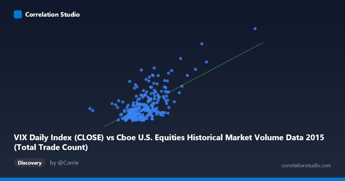
VIX Daily Index (CLOSE) vs Cboe U.S. Equities Historical Market Volume Data 2015 (Total Trade Count)

Pearson correlation (r): 0.6459
Spearman correlation: 0.5266
p-value: 0
Sample size (n): 252
95% confidence interval: 0.5677 to 0.7126
Granger causality: None
Granger optimal lag: 1

AI analysis

Scatterplot Analysis: VIX vs. Total Trade Count (2015)

Relationship Overview The scatterplot reveals a moderate positive relationship between the CBOE Volatility Index (VIX) daily close values and total trade counts on U.S. equities exchanges throughout 2015. As VIX levels rise — indicating greater market fear or uncertainty — trading activity as measured by total trade counts tends to increase correspondingly. This is an intuitively sensible relationship: periods of elevated volatility typically drive heightened market participation as traders react, hedge, or reposition. The linear regression equation (y = 6.019×10⁻⁶x + 1.712) suggests a shallow but meaningful positive slope across the observed range.

Correlation Strength and Statistical Significance The correlation coefficient of r = 0.646 indicates a moderate-to-strong positive association, with r² = 0.417 meaning that approximately 41.7% of the variance in trade counts is explained by VIX levels — a practically meaningful but incomplete picture, leaving roughly 58% of variance attributable to other factors. The 95% confidence interval of [0.568, 0.713] is relatively tight given the sample of n = 252, and the p-value of effectively zero confirms this relationship is highly unlikely to be a statistical artifact. However, Granger causality tests reveal no significant temporal predictive direction in either direction (X→Y: F = 0.105, p = 0.746; Y→X: F = 0.090, p = 0.764), meaning that while the two variables are strongly contemporaneously correlated, neither reliably predicts the other at a one-period lag. This is a critical distinction: correlation here is likely driven by shared simultaneous responses to market events rather than one variable driving the other sequentially.

Notable Patterns, Clusters, and Outliers The sample points reveal a dense central cluster concentrated in the X range of roughly 1,800,000–2,700,000 and Y range of 12–20, suggesting that the majority of 2015 trading days were characterized by moderate volatility and moderate trade activity. However, there is a visible upper-right tail of notable outliers — points such as (4,083,022, 36.02) and (3,907,921, 28.03) — representing days of extreme volatility paired with very high trade counts, likely corresponding to the August 2015 market correction. These high-leverage points likely exert disproportionate influence on the regression slope and correlation coefficient. The distribution also appears somewhat heteroscedastic, with variance in trade counts widening considerably at higher VIX levels, suggesting the relationship is not uniformly consistent across all volatility regimes.

Confounding Factors and Caveats Several confounding factors complicate causal interpretation. First, both VIX and trade volume are likely jointly driven by common macroeconomic or news shocks — such as Federal Reserve announcements, geopolitical events, or earnings seasons — rather than one causing the other, which aligns with the Granger causality null result. Second, the 2015 timeframe includes the August flash crash, which may artificially inflate the correlation by introducing a few extreme co-movement events that dominate the statistical relationship. Third, structural market factors such as algorithmic trading, exchange-specific quirks, and intraday circuit breakers could influence trade counts independently of volatility. It is also worth noting that the axis labels appear swapped in the metadata (VIX is listed as the X-axis source but labeled as a Y-axis dataset and vice versa), which warrants verification before drawing firm conclusions.

Actionable Insights and Further Investigation Practitioners could use this relationship as a regime indicator: elevated VIX levels can serve as a rough proxy for expecting heightened trading activity, which has implications for liquidity management, execution strategy, and market impact modeling. For further investigation, it would be valuable to: (1) segment the analysis by market regime (e.g., VIX < 15 vs. VIX 20) to test whether the relationship holds differently in calm vs. stressed environments; (2) apply rolling correlations to assess whether the relationship was stable throughout 2015 or concentrated in the August volatility episode; (3) include additional covariates such as S&P 500 returns, bid-ask spreads, or options volume to build a more complete explanatory model; and (4) extend the dataset beyond 2015 to test whether this correlation generalizes across multiple market cycles or is period-specific.

X dataset: Cboe U.S. Equities Historical Market Volume Data 2015

Y dataset: VIX Daily Index

Part of experiment: Daily - Cboe U.S. Equities Historical Market Volume Data 2015 vs VIX Daily Index