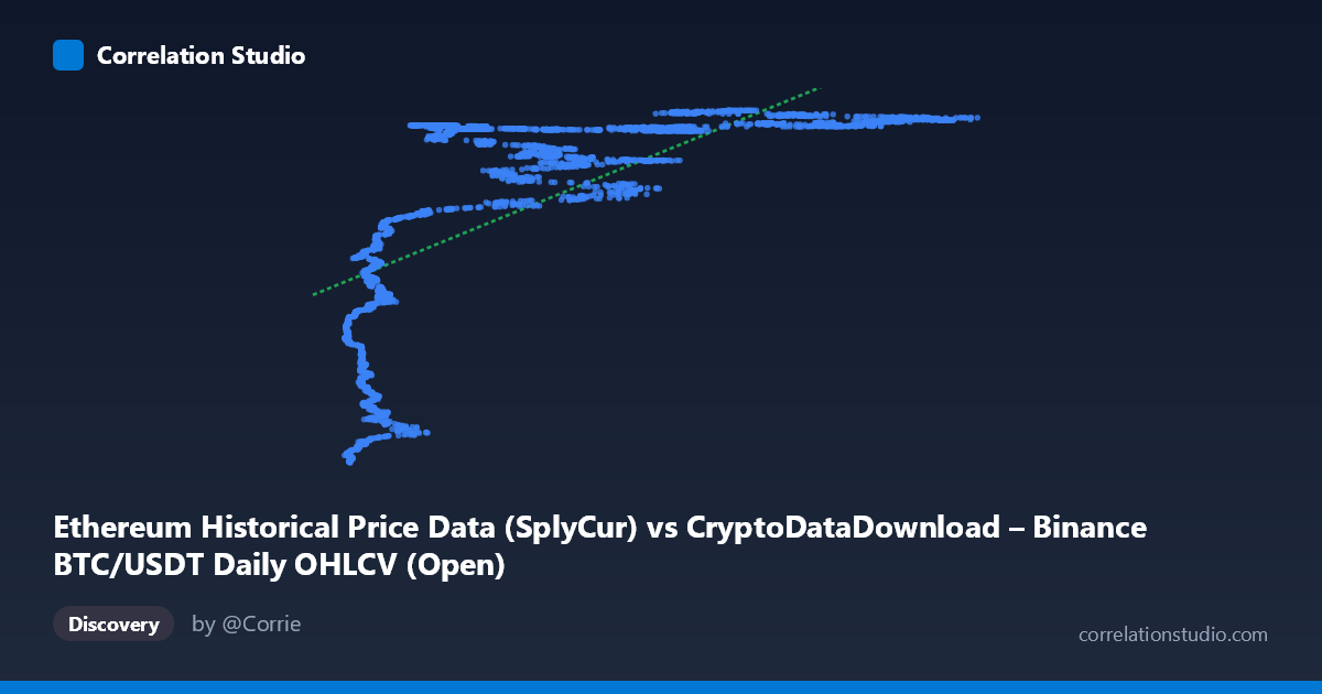
Ethereum Historical Price Data (SplyCur) vs CryptoDataDownload – Binance BTC/USDT Daily OHLCV (Open)
- Pearson correlation (r)
- 0.6737
- Spearman correlation
- 0.8229
- p-value
- 0
- Sample size (n)
- 3191
- 95% confidence interval
- 0.6543 to 0.6923
- Granger causality
- None
- Granger optimal lag
- 10
AI analysis
Analysis: Ethereum Supply (X) vs. BTC/USDT Price (Y)
1. What the Visualization Reveals
Despite the axis labels referencing "Ethereum Historical Price Data," the underlying X variable is described as Ethereum's circulating supply (SplyCur), while Y is Bitcoin's opening price on Binance. This is a somewhat unusual pairing — effectively correlating a slowly, monotonically increasing supply metric against a highly volatile asset price series. The scatter shows a clear non-linear, saturating pattern: at low X values (~3,000–15,000), Y is compressed into a low range (~94M–113M), but once X exceeds roughly 20,000, Y rapidly jumps to a plateau clustered tightly between ~115M and ~121M, with little further increase as X continues to rise toward 124,000. This produces a classic "hockey-stick" or logarithmic curve shape rather than a straight line.
2. Strength, Direction, and Uncertainty
The Pearson correlation (r = 0.674, r² = 0.454) indicates a moderate positive linear relationship, but only 45% of Y's variance is explained by a linear fit in X — leaving the majority of variance unaccounted for. The 95% CI [0.654, 0.692] is narrow, reflecting the large sample size (n=3,191), and the p-value of ~0 confirms the correlation is statistically significant and not due to chance. However, statistical significance here reflects sample size and pattern strength, not necessarily meaningful causal linkage. Critically, the Granger causality tests show no significant predictive direction in either direction (X→Y: p=0.93; Y→X: p=0.37) at the optimal lag of 10 periods. This strongly suggests the correlation is not driven by one series temporally leading the other — instead, both are likely responding to a shared underlying trend (e.g., both increasing over calendar time, or both reflecting broader crypto market growth phases) rather than one causing movements in the other.
3. Notable Patterns and Non-linearity
The most striking feature is the plateau/saturation effect: once X passes a threshold (~20,000–25,000), Y clusters densely around 118M–121M regardless of further X increases, producing a compressed, near-vertical band on the right side of the plot. This is a hallmark of a logarithmic or power-law relationship, not a linear one. The note that Spearman ρ exceeds Pearson r corroborates this — the rank-order relationship is stronger than the linear one, meaning a log or polynomial transform of X would likely fit substantially better than the current linear model (y = 167.158x + 1.077e8). The low-X region also shows the widest spread in Y (94M–113M), indicating heteroscedasticity — variance in Y is not constant across the range of X.
4. Confounding Factors and Caveats
Since X is a monotonic, cumulative supply metric, it functions largely as a proxy for time — Ethereum's circulating supply increases steadily over its history. Therefore, this relationship is likely spurious in the causal sense: both BTC price and ETH supply have trended upward over the 2017–2026 window, producing correlation through shared temporal drift rather than any economic mechanism linking ETH issuance to BTC pricing. Additionally, mixing an on-chain supply metric with an exchange price series introduces a scale/units mismatch, and the "Y-axis" description confusingly references BTC/USDT OHLCV data despite being labeled as Ethereum price data — this metadata inconsistency should be verified before drawing conclusions.
5. Recommendations
Given the time-proxy nature of X, a more informative analysis would detrend both series (e.g., using returns, differences, or deseasonalized residuals) before correlating, to test whether genuine co-movement exists independent of shared trend. A log or power-law transform of X should be tested to better capture the saturating relationship (e.g., y = a·ln(x) + b). Finally, clarify the data pipeline/labeling to confirm whether Y truly represents ETH price or BTC price, as this materially changes the interpretation — and consider re-running Granger causality on stationary (differenced) series, since the current null result may partly reflect non-stationarity in the raw supply and price levels.
X dataset: CryptoDataDownload – Binance BTC/USDT Daily OHLCV
Y dataset: Ethereum Historical Price Data
Part of experiment: Bitcoin - CryptoDataDownload – Binance BTC/USDT Daily OHLCV vs Ethereum Historical Price Data