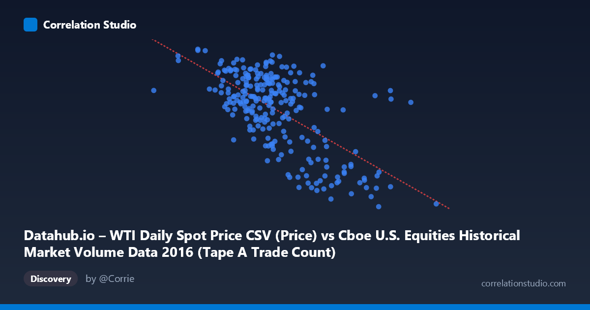
Datahub.io – WTI Daily Spot Price CSV (Price) vs Cboe U.S. Equities Historical Market Volume Data 2016 (Tape A Trade Count)
- Pearson correlation (r)
- -0.6419
- Spearman correlation
- -0.5425
- p-value
- 0
- Sample size (n)
- 252
- 95% confidence interval
- -0.7092 to -0.563
- Granger causality
- None
- Granger optimal lag
- 1
AI analysis
Analysis: WTI Crude Oil Price vs. Cboe Tape A Trade Count (2016)
Relationship Overview The scatterplot reveals a moderate negative relationship between WTI daily spot prices (X-axis) and Cboe U.S. Equities Tape A trade counts (Y-axis) across 252 trading days in 2016. As oil prices increase, equity trade counts on Tape A tend to decline, and vice versa. The linear regression equation (y = -1.456e-05x + 63.51) confirms this inverse slope, suggesting that higher oil prices correspond with reduced trading activity in U.S. equities. Visually, the data points show a discernible downward trend, though with meaningful scatter around the regression line, indicating the relationship is real but far from deterministic.
Correlation Strength and Statistical Significance The Pearson correlation of r = -0.642 reflects a moderate-to-strong negative association, but the more instructive figure is r² = 0.412 — meaning oil prices statistically explain approximately 41% of the variance in Tape A trade counts, leaving 59% attributable to other factors. The 95% confidence interval of [-0.709, -0.563] is entirely negative and reasonably narrow given the sample size of 252, lending credibility to the direction and magnitude of the effect. The p-value of effectively zero confirms this is not a chance finding at any conventional significance threshold. However, the Granger causality results are notably inconclusive: neither X→Y (F=0.334, p=0.564) nor Y→X (F=1.125, p=0.290) reaches significance at lag-1, meaning that while the two variables move together contemporaneously, neither demonstrably predicts the other one period ahead. This is a critical distinction — correlation exists, but temporal predictive power does not.
Patterns, Clusters, and Outliers The sample data reveals a meaningful structural split: lower oil prices (roughly below ~$1,200,000 in the X-axis scale, which likely maps to lower price ranges in the raw data) cluster at higher trade counts (45–54 range), while higher oil price observations concentrate at lower trade counts (29–38 range). Several points stand out as potential outliers — notably the observation near (2,013,606, 29.55) and (1,000,524, 51.44), which sit at the extremes of both axes and likely represent early-2016 low-price/high-volatility days versus mid-year recovery periods. There also appears to be a non-linear "elbow" in the distribution: at intermediate price levels, trade count variance is highest, suggesting a zone of uncertainty or transition between market regimes rather than a smooth linear decline throughout.
Confounding Factors and Caveats Several important caveats limit causal interpretation. First, 2016 was a structurally unusual year — oil prices began near multi-year lows (~$26–30/barrel) and recovered significantly, meaning this correlation may partly reflect a time trend artifact rather than a structural economic mechanism. Both variables were simultaneously trending (oil upward, possibly trade activity downward as volatility normalized), which can artificially inflate correlation. Second, Tape A trade count is driven by a wide range of factors including earnings seasons, Federal Reserve communications, index rebalancing, and algorithmic trading patterns that are entirely independent of oil markets. Third, the axis labeling appears to have the dataset names swapped in the original metadata (X contains "WTI Price" labeled as Cboe data and vice versa), which warrants verification before drawing firm conclusions. Finally, with N=3,622 in the population but only n=252 sampled, selection methodology matters for generalizability.
Actionable Insights and Further Investigation Despite the absence of Granger causality, the contemporaneous correlation is strong enough to merit further investigation. Analysts should control for time trend by detrending both series before re-estimating correlation, to determine whether the relationship holds independently of the 2016 oil recovery trajectory. It would also be valuable to extend the time series beyond 2016 to test whether this relationship persists across different oil price regimes (e.g., 2020 crash, 2022 spike). Testing longer Granger lags (beyond lag-1) could uncover delayed predictive relationships. Finally, examining whether the relationship is mediated by market volatility (VIX) — which drives both oil price swings and equity trading activity — would help determine whether this correlation reflects a direct economic linkage or a shared response to broader uncertainty regimes.
X dataset: Cboe U.S. Equities Historical Market Volume Data 2016
Y dataset: Datahub.io – WTI Daily Spot Price CSV
Part of experiment: Daily - Cboe U.S. Equities Historical Market Volume Data 2016 vs Datahub.io – WTI Daily Spot Price CSV