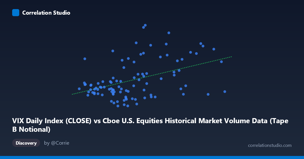
VIX Daily Index (CLOSE) vs Cboe U.S. Equities Historical Market Volume Data (Tape B Notional)

Pearson correlation (r): 0.4299
Spearman correlation: 0.3403
p-value: 0.000009
Sample size (n): 99
95% confidence interval: 0.254 to 0.5782
Granger causality: None
Granger optimal lag: 1

AI analysis

Scatterplot Analysis: Market Volume (Tape B Notional) vs. VIX Daily Index

Overall Relationship The scatterplot reveals a moderate positive relationship between Cboe U.S. Equities market volume (Tape B Notional, on the X-axis) and the VIX Daily Index (Y-axis) over the January–May 2026 period. As trading volume in Tape B increases, VIX levels tend to rise, which aligns intuitively with the well-established financial narrative that heightened market activity often accompanies elevated uncertainty or volatility. The linear regression equation (y = 5.075×10⁻¹⁰x + 13.62) confirms this positive slope, though the relationship is far from deterministic, as evidenced by the considerable scatter around the fitted line.

Correlation Strength and Statistical Significance The Pearson correlation of r = 0.43 indicates a moderate positive association, but the explanatory power is notably limited: r² = 0.185, meaning only about 18.5% of the variance in VIX is explained by Tape B volume. The remaining ~81.5% of VIX variability is driven by other factors entirely. The 95% confidence interval for r [0.254, 0.578] is meaningfully above zero throughout, and the p-value of 8.97×10⁻⁶ confirms this correlation is highly statistically significant — unlikely to be a chance artifact. However, statistical significance must not be conflated with practical magnitude; this is a weak-to-moderate effect at best. Critically, the Granger causality tests reveal no significant temporal predictive direction in either direction (X→Y: F=0.003, p=0.956; Y→X: F=0.003, p=0.959). Neither variable reliably predicts the other's future values, which substantially tempers any causal interpretation. The correlation reflects co-movement, not a forecasting relationship.

Notable Patterns, Clusters, and Outliers The point cloud shows substantial heteroscedasticity — scatter appears to widen at higher volume levels, suggesting the relationship becomes less predictable as volumes increase. Several notable outliers are visible: the point at approximately (13.4B, 31.05) sits far above the regression line and represents an extreme VIX spike on relatively moderate volume, while (13.2B, 30.61) similarly clusters in an anomalously high VIX region. Conversely, points such as (19.4B, 16.88) and (20.98B, 17.44) represent very high volume days with surprisingly subdued VIX readings, suggesting that volume spikes can occur in low-volatility environments (e.g., passive rebalancing or index events). There appears to be a loose cluster of lower-volume, moderate-VIX observations (roughly 8–12B volume, VIX 16–20) forming a dense core, with higher-volume observations more dispersed at elevated VIX values.

Confounding Factors and Caveats Several important caveats apply. First, dataset labeling appears reversed — the X-axis is labeled "VIX Daily Index (CLOSE)" from the market volume dataset, and the Y-axis as "Tape B Notional" from the VIX dataset, suggesting a metadata mismatch that warrants verification before drawing firm conclusions. Second, the N=1,980 population size vs. n=99 sample means this analysis covers roughly 5% of the available data; while the sample is likely representative, seasonal effects within a single year (Jan–May 2026) may introduce temporal autocorrelation that inflates apparent significance. Third, macroeconomic events (earnings seasons, Fed policy announcements, geopolitical developments) could simultaneously drive both volume and VIX, acting as common confounders. The Granger causality null result reinforces that any correlation here is likely contemporaneous co-movement driven by shared external shocks rather than one variable driving the other.

Actionable Insights and Further Investigation Given the modest explanatory power and absence of Granger causality, practitioners should avoid using Tape B volume alone as a VIX forecasting signal. More productive next steps would include: (1) decomposing volume by trade type (institutional block trades vs. retail flow) to identify whether specific volume components carry stronger VIX predictive power; (2) testing non-linear models (e.g., quadratic or regime-switching) given the apparent heteroscedasticity and the presence of extreme outliers that may reflect distinct market regimes; (3) expanding the time window beyond early 2026 to assess whether this moderate correlation is stable across bull/bear cycles or is period-specific; and (4) investigating the extreme outlier dates (e.g., the ~31 VIX spike at moderate volume) for event-driven explanations that may represent structurally different observations worth excluding or modeling separately.

X dataset: Cboe U.S. Equities Historical Market Volume Data

Y dataset: VIX Daily Index

Part of experiment: Daily - Cboe U.S. Equities Historical Market Volume Data vs VIX Daily Index