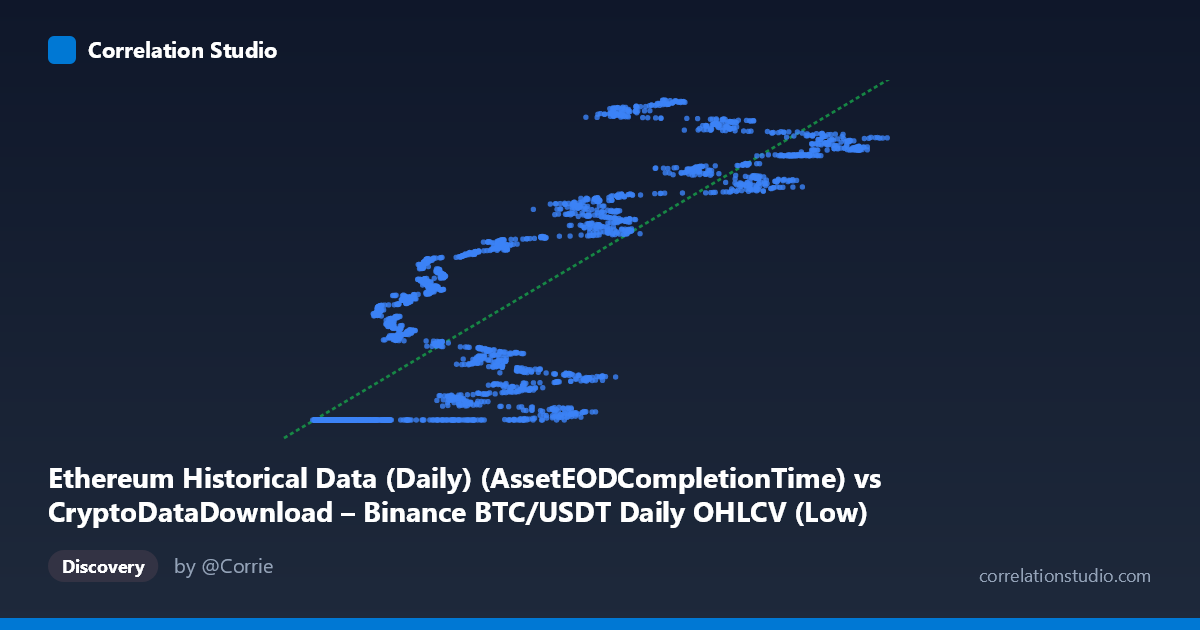
Ethereum Historical Data (Daily) (AssetEODCompletionTime) vs CryptoDataDownload – Binance BTC/USDT Daily OHLCV (Low)
- Pearson correlation (r)
- 0.8552
- Spearman correlation
- 0.89
- p-value
- 0
- Sample size (n)
- 3191
- 95% confidence interval
- 0.8456 to 0.8642
- Granger causality
- None
- Granger optimal lag
- 10
- Time coverage
- 2017-08-17 to 2026-05-20
AI analysis
Analysis: BTC/USDT vs. Ethereum Historical Data Scatterplot
1. Relationship Overview
The scatterplot depicts a strong, positive, non-linear relationship between the two variables, though the underlying data labeling appears mismatched (the X-axis is nominally a timestamp field while Y is a price/low value). Practically, this plot behaves like a time-versus-price chart rather than a relationship between two independent economic variables. The pattern shows a clear "step" structure: a large cluster of points at the minimum Y value (~1,614,335,300) spanning X values from ~2,800 to ~35,000, followed by a sharp upward transition to a much higher, more scattered band of Y values (1,660,000,000–1,780,000,000) for X 35,000.
2. Strength, Direction, and Uncertainty
The Pearson correlation (r = 0.8552, r² = 0.7313) indicates a strong positive association, with roughly 73% of the variance in Y statistically explained by X in a linear framework. The 95% CI [0.8456, 0.8642] is tight, and the p-value is effectively zero, meaning the correlation is highly unlikely to be due to random chance given this sample. However, this strength is misleading: the relationship is clearly not linear — it's a threshold/step function — so the linear r² substantially understates how deterministic the low-X segment is (nearly constant Y) while overstating the linear fit's descriptive accuracy for the high-X segment (which is noisy and heteroscedastic). Critically, the Granger causality tests show no significant predictive direction in either direction (X→Y: p=0.357; Y→X: p=0.190). This tells us that despite the strong contemporaneous correlation, neither variable helps forecast the other's future values beyond its own history — the relationship is likely driven by a shared external factor (e.g., calendar time or a common market regime) rather than one variable causing changes in the other.
3. Notable Patterns and Outliers
Three distinct regimes are visible: - Flat baseline cluster (X < 35,000): Y is pinned near 1,614,335,300 with almost zero variance — this looks like a data artifact (a placeholder/minimum value) rather than genuine market data, since real price series rarely stay perfectly flat for thousands of points. - Transition zone (X ≈ 35,000–60,000): Y begins rising and becomes volatile, with values like 1,619,059,610 and 1,642,814,716 showing the "escape" from the floor. - Upper scattered band (X 60,000): Y fluctuates between ~1,700,000,000 and ~1,780,000,000 with no clear increasing trend relative to X — this looks like noise around a new elevated baseline, not continued linear growth.
This step-like shape strongly resembles a regime shift (e.g., a data recording change, a market structural break, or units/definition change mid-series) rather than smooth co-movement.
4. Confounding Factors and Caveats
Several caveats are essential: - Field mismatch/likely data error: The X-axis is described as a timestamp column, and Y as a "Low" price — but Y values (~1.6–1.8 billion) don't correspond to realistic BTC or ETH price levels, suggesting Y may itself be an epoch timestamp or a miscoded field. This should be verified before drawing market conclusions. - Autocorrelation: Both series are highly autocorrelated over time (typical of price/time data), which inflates apparent correlation and violates the independence assumption behind standard p-values — the "N=3,212 independent observations" is likely overstated in effective degrees of freedom. - Non-stationarity: The flat-then-rising structure suggests non-stationary behavior, which can produce spurious high correlations between otherwise unrelated series (a classic time-series pitfall). - No causal mechanism confirmed: The lack of Granger causality reinforces that this correlation should not be interpreted as one asset driving the other's price.
5. Recommendations for Further Investigation
1. Verify data integrity — confirm whether the X and Y columns are correctly mapped and whether the "flat" segment reflects a real data collection gap, padding, or default value rather than genuine market inactivity. 2. Difference or detrend both series (e.g., use daily returns instead of raw levels) before recomputing correlation — this will reveal whether co-movement persists after removing shared trend/non-stationarity, a more rigorous test than raw-level Pearson r. 3. Segment the analysis into the flat-baseline period and the volatile period separately, since pooling both regimes distorts both the correlation coefficient and the regression slope. 4. Test for a shared third factor (e.g., overall crypto market cap, BTC dominance, or exchange-wide volume) that might explain co-movement without direct causality between the two named variables. 5. Given no Granger causality, avoid using either series to forecast the other; instead, treat the strong r² as evidence of common trend/regime alignment, not predictive power.
X dataset: CryptoDataDownload – Binance BTC/USDT Daily OHLCV
Y dataset: Ethereum Historical Data (Daily)
Part of experiment: Bitcoin - CryptoDataDownload – Binance BTC/USDT Daily OHLCV vs Ethereum Historical Data (Daily)