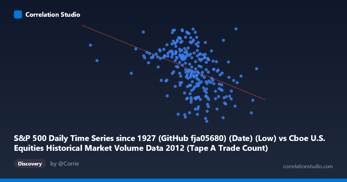
S&P 500 Daily Time Series since 1927 (GitHub fja05680) (Date) (Low) vs Cboe U.S. Equities Historical Market Volume Data 2012 (Tape A Trade Count)
- Pearson correlation (r)
- -0.4172
- Spearman correlation
- -0.4757
- p-value
- 0
- Sample size (n)
- 250
- 95% confidence interval
- -0.5146 to -0.3091
- Granger causality
- None
- Granger optimal lag
- 2
AI analysis
Analysis: S&P 500 Daily Low vs. Cboe Tape A Trade Count (2012)
Relationship Overview The scatterplot reveals a moderate negative relationship between the S&P 500 daily low price (X-axis) and Cboe Tape A trade count (Y-axis) across the 2012 trading year. As the S&P 500 daily low increases — reflecting rising equity valuations — the number of individual trades on Tape A tends to decline. This is an intuitively meaningful finding: during periods of lower prices (often associated with market stress or uncertainty), traders tend to execute more frequent, smaller transactions, whereas rising markets tend to see consolidation of trading activity into fewer, larger orders. The linear regression equation (y = −0.000137x + 1508.54) quantifies this inverse slope, though the relationship is far from deterministic across the observed range of roughly 350,000 to 1,423,000 for X and 1,259 to 1,460 (in thousands) for Y.
Correlation Strength, Uncertainty, and Temporal Direction The Pearson correlation of r = −0.4172 indicates a moderate negative association, but the coefficient of determination r² = 0.1741 is the more sobering figure — it means that only about 17.4% of the variance in Tape A trade count is explained by the S&P 500 daily low. The remaining ~82.6% of variance is attributable to other factors entirely. Despite this modest explanatory power, the statistical significance is unambiguous: the p-value of 5.99 × 10⁻¹² with n = 250 paired observations drawn from a population of 3,750 confirms this is not a chance finding, and the 95% confidence interval of [−0.515, −0.309] is comfortably negative throughout, indicating reliable directionality even if the magnitude remains uncertain. Critically, the Granger causality tests reveal no significant predictive directionality in either direction — neither X→Y (F = 2.04, p = 0.133) nor Y→X (F = 0.56, p = 0.575) achieves significance at conventional thresholds with an optimal lag of 2 periods. This means that while the two variables are correlated contemporaneously, past values of the S&P 500 low do not reliably predict future trade counts, and vice versa, cautioning against any causal or predictive trading strategy built on this relationship alone.
Patterns, Clusters, and Outliers The scatterplot exhibits notable heteroscedasticity and clustering. In the lower X range (S&P 500 lows below ~850,000), trade counts span a relatively wide band between approximately 1,350 and 1,460, suggesting high variability in trading activity during lower-valuation periods. As the index low rises above ~1,100,000, the distribution tightens but shifts downward in Y, with most observations clustering between 1,280 and 1,420. Several potential outliers are visible: the point near (1,290,790; 1,460.07) is notable as both an extreme X value and an unusually high Y value, defying the overall trend, while points such as (959,328; 1,273.34) and (964,117; 1,268.10) represent anomalously low trade counts relative to their X position. These outliers may correspond to specific calendar events — holidays, options expiration days, or macro announcements — that temporarily disrupted normal trading patterns.
Confounding Factors and Interpretive Caveats Several important confounds complicate a straightforward interpretation. Market microstructure changes in 2012 — including algorithmic trading surges, regulatory interventions, and exchange fee adjustments — could independently drive trade counts regardless of price levels. The day-of-week and month-of-year effects (e.g., lower volume in summer months, higher volume around earnings seasons) create seasonal autocorrelation that may inflate or distort the apparent correlation. Additionally, the denominator mismatch is worth flagging: the X variable is a price level (S&P 500 daily low), which drifted broadly upward through 2012 as markets recovered, while Tape A trade count reflects structural exchange-level activity that is influenced by fragmentation across venues, dark pools, and TRFs simultaneously. The absence of Granger causality also underscores that this correlation is likely a shared response to common underlying drivers — macroeconomic sentiment, volatility regimes (VIX), and liquidity conditions — rather than a direct mechanistic link.
Actionable Insights and Further Investigation Practitioners and researchers should pursue several avenues to enrich this analysis. First, incorporating realized volatility or VIX as a control variable would test whether the negative correlation persists after accounting for risk-appetite regimes, which likely drive both price levels and trade fragmentation simultaneously. Second, segmenting the data by market regime (e.g., trend days vs. range-bound days, pre/post Federal Reserve announcements) could reveal whether the correlation is driven by specific subperiods rather than being a stable structural feature. Third, extending the analysis to other Tape designations (B and C) and comparing fragmentation patterns would clarify whether this is a Cboe-specific phenomenon or a market-wide dynamic. Finally, given the non-significant Granger causality, a VAR model with additional covariates (volume, bid-ask spreads, options activity) may better capture the multivariate dynamics that the bivariate framework leaves unexplained in its substantial residual 82.6% variance.
X dataset: Cboe U.S. Equities Historical Market Volume Data 2012
Y dataset: S&P 500 Daily Time Series since 1927 (GitHub fja05680) (Date)
Part of experiment: Daily - Cboe U.S. Equities Historical Market Volume Data 2012 vs S&P 500 Daily Time Series since 1927 (GitHub fja05680) (Date)