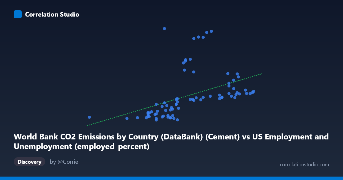
World Bank CO2 Emissions by Country (DataBank) (Cement) vs US Employment and Unemployment (employed_percent)
- Pearson correlation (r)
- 0.442
- Spearman correlation
- 0.742
- p-value
- 0.000041
- Sample size (n)
- 80
- 95% confidence interval
- 0.2462 to 0.6031
- Granger causality
- None
- Granger optimal lag
- 10
AI analysis
Scatterplot Analysis: Cement CO2 Emissions vs. US Employment Percentage
1. Overall Relationship
The scatterplot reveals a positive but weak-to-moderate relationship between World Bank cement CO2 emissions and the US employed percentage, spanning data from 1941 to 2020. The linear regression equation (y = 96.48x − 4921.68) indicates that higher cement CO2 emissions associate with higher US employment percentages, but the scatter around this trend line is substantial. Visually, the data does not form a tight band — instead, points are broadly dispersed, suggesting that the linear model captures only a fraction of the underlying dynamics. The wide Y-axis range (78.58 to 2608.93) relative to the narrower X-axis range (50.40 to 64.40) immediately signals high variability in CO2 emissions even within narrow employment ranges, hinting at complexity beyond a simple linear story.
2. Correlation Strength, Direction, and Temporal Causality
The Pearson correlation of r = 0.4420 indicates a moderate positive association, but the explanatory power is modest: r² = 0.1953 means only ~19.5% of variance in CO2 cement emissions is explained by US employment percentage. The remaining ~80.5% is attributable to other factors entirely outside this model. The 95% confidence interval for r of [0.2462, 0.6031] is relatively wide, reflecting meaningful uncertainty — while the lower bound confirms a genuine positive association, the upper bound falls well short of a strong correlation. The p-value of 4.05×10⁻⁵ confirms the result is statistically significant (far below α = 0.05), so we can confidently reject the null hypothesis of no linear relationship. However, statistical significance here is partly a function of the reasonably large sample (n = 80). Critically, Granger causality testing finds no significant predictive directionality in either direction — neither X→Y (F = 0.505, p = 0.878) nor Y→X (F = 1.729, p = 0.101) — meaning that past values of employment do not reliably predict future cement CO2 levels, and vice versa, even at the optimal lag of 10 periods. This substantially limits any causal narrative and suggests the observed correlation may be largely coincidental or driven by shared confounders rather than a direct mechanistic link.
3. Notable Patterns, Clusters, and Outliers
Several features stand out visually. There is a cluster of lower employment values (55–58%) paired with relatively low CO2 emissions (roughly 100–650 units), forming a dense lower-left grouping. A second, more diffuse cluster appears at higher employment rates (59–64%) with moderate-to-high CO2 values (700–1400 units). Most strikingly, there are notable outliers with extreme Y-values: points like (56.80, 2608.93), (60.80, 2532.94), (60.40, 2501.79), (59.70, 2374.89), and (59.30, 2333.75) show very high cement CO2 emissions paired with only moderate employment percentages — these high-leverage points likely exert disproportionate influence on the regression line. The fact that Spearman ρ exceeds Pearson r further confirms a non-linear or rank-distorted relationship, suggesting these extreme values distort the linear fit and that a polynomial or logarithmic transformation of Y might better capture the true association.
4. Confounding Factors and Caveats
Several important caveats apply. First, this correlation conflates two conceptually mismatched datasets — global cement CO2 emissions (a worldwide aggregate) and US employment percentage (a domestic labor statistic) — making any direct causal interpretation immediately suspect. Both variables are likely driven by common global or US macroeconomic cycles: periods of economic expansion drive both higher US employment and greater global construction/cement demand simultaneously, creating a spurious correlation. Second, the 80-year time span (1941–2020) introduces substantial structural breaks — World War II mobilization, post-war industrialization, the 1970s oil shocks, deindustrialization, and the 2008 financial crisis — each of which would affect both variables independently. Third, the extreme outliers identified above may correspond to specific economic shocks or data anomalies (e.g., pandemic-era disruptions in 2020) that deserve individual investigation rather than being smoothed into a regression line. Finally, using annual aggregates masks seasonal and sub-annual dynamics that could clarify or dissolve the apparent relationship.
5. Actionable Insights and Further Investigation
Given these findings, several next steps are warranted. Apply a log or polynomial transformation to Y (CO2 cement emissions) to address the right-skewed distribution and non-linearity flagged by the Spearman-Pearson discrepancy — this may yield a tighter, more interpretable fit. Investigate the high-emission outliers individually to determine whether they correspond to specific historical events (e.g., post-recession construction booms, data revisions, or geopolitical shifts in cement production). A multiple regression approach incorporating GDP growth, global construction indices, or energy prices would likely absorb much of the unexplained 80.5% variance and reveal whether the employment-CO2 link survives controls. Since Granger causality finds no temporal predictive relationship, researchers should shift focus from predictive modeling to structural equation modeling that accounts for shared economic drivers. Finally, disaggregating the analysis by decade could reveal whether the correlation strengthened or weakened over time, particularly given the dramatic shifts in US manufacturing and global cement production geography since the 1980s.
X dataset: US Employment and Unemployment
Y dataset: World Bank CO2 Emissions by Country (DataBank)
Part of experiment: Yearly - US Employment and Unemployment vs World Bank CO2 Emissions by Country (DataBank)