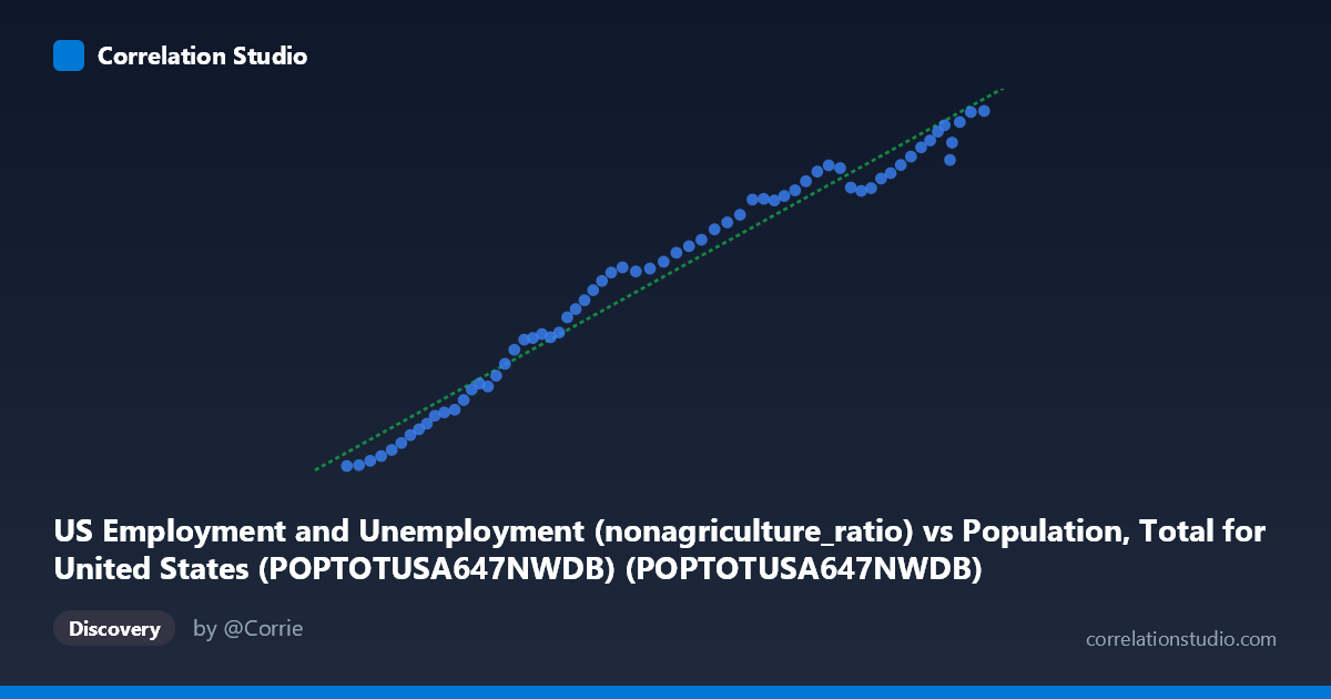
US Employment and Unemployment (nonagriculture_ratio) vs Population, Total for United States (POPTOTUSA647NWDB) (POPTOTUSA647NWDB)
- Pearson correlation (r)
- 0.9858
- Spearman correlation
- 0.9949
- p-value
- 0
- Sample size (n)
- 65
- 95% confidence interval
- 0.9767 to 0.9913
- Granger causality
- None
- Granger optimal lag
- 10
- Time coverage
- 1960-01-01 to 2024-01-01
AI analysis
Analysis: US Population vs. Non-Agricultural Employment Ratio
1. Overall Relationship The scatterplot reveals a strikingly strong, positive, and nearly linear relationship between total US population and the non-agricultural employment ratio. As population grows from approximately 180.7 million to 340.1 million across the 1960–2024 period, the employment metric rises correspondingly from roughly 60,318 to 159,091. The data points trace what appears to be a smooth, continuous arc with minimal scatter around the regression line (y = 0.000617x − 47,455.9), suggesting that these two variables have moved in near-lockstep over six decades of American demographic and economic history.
2. Correlation Strength and Statistical Interpretation The correlation is exceptionally strong at r = 0.9858, and the coefficient of determination r² = 0.9718 means that approximately 97.2% of the variance in the non-agricultural employment figure is statistically explained by variation in total population. The 95% confidence interval [0.9767, 0.9913] is remarkably narrow, indicating high precision in the estimate, and the p-value of effectively zero confirms this relationship is not a chance artifact. However, the Granger causality results tell a more cautionary tale: neither X→Y (F = 0.4960, p = 0.8806) nor Y→X (F = 0.3881, p = 0.9431) achieves significance at any conventional threshold, even at an optimal lag of 10 periods. This means that despite the near-perfect contemporaneous correlation, neither variable meaningfully predicts future changes in the other beyond what a simple time trend already captures — a classic signature of spurious correlation driven by shared secular trends.
3. Notable Patterns, Clusters, and Outliers The data points fall into loosely distinguishable clusters reflecting different eras. Earlier observations (1960s–1970s, lower-left quadrant, X ≈ 180–230M) exhibit a slightly steeper slope-per-unit relationship, while mid-range points (1980s–2000s) show steady linear progression. The upper-right cluster (X 310M, post-2010) appears marginally compressed in Y-growth relative to the regression line, possibly reflecting labor force participation rate changes in recent years. No dramatic outliers are visible, though a few points near X ≈ 330–340M show slight divergence, potentially reflecting pandemic-era labor market disruptions around 2020–2022. The overall smoothness of the trajectory is itself noteworthy — it reflects the slow-moving, trend-dominated nature of both variables.
4. Confounding Factors and Interpretive Caveats The most critical caveat is that both variables are primarily driven by the passage of time. Population grows quasi-monotonically due to births, immigration, and declining mortality. Non-agricultural employment similarly grows as the economy expands. The correlation therefore largely captures a shared upward time trend rather than a direct causal mechanism linking population size to employment levels. Confounders include GDP growth, technological change, female labor force entry (especially post-1960s), immigration policy, cyclical recessions, and structural economic shifts toward services. The Granger test failure confirms that once time-trend structure is accounted for, no additional predictive information flows between the two series. The regression equation itself (negative intercept of −47,456) is economically uninterpretable at face value, further signaling a trend-based artifact.
5. Actionable Insights and Further Investigation Researchers should detrend both series (e.g., using first differences, percentage changes, or HP filtering) before drawing conclusions about a structural relationship between population and employment. It would be valuable to examine the employment-to-population ratio directly, or to investigate specific demographic subgroups (prime-age workers, 25–54) to identify whether population composition — not just size — drives employment dynamics. Testing against alternative drivers such as GDP per capita, real wages, or sector-specific employment shares would help disentangle genuine economic relationships from trend coincidence. Additionally, examining recession years as structural breakpoints (2001, 2008–09, 2020) could reveal whether the relationship weakens under economic stress, which would be analytically meaningful for labor market policy modeling.
X dataset: Population, Total for United States (POPTOTUSA647NWDB)
Y dataset: US Employment and Unemployment
Part of experiment: Yearly - Population, Total for United States (POPTOTUSA647NWDB) vs US Employment and Unemployment